Intensity Mapping

21 cm cosmology studies the redshifted 21 cm-wavelength photons that are emitted in a hyperfine transition of atomic hydrogen atoms (HI). The transition occurs when an electron in the excited spin triplet state flips its spin relative to the proton and falls into the singlet state. While this transition is quantum mechanically “forbidden” to first order, a very large number of neutral hydrogen atoms in massive clouds render the signal observable.

The hyperfine transition can be used to trace the matter field through a technique called 21 cm intensity mapping (IM) (Santos et al. 2015). It is possible since the spin transition in HI is optically thin (Furlanetto et al. 2006), meaning that 21 cm photons are unlikely to be absorbed/emitted more than once as they travel to our telescopes. Therefore, full 3D mappings of the 21 cm line become possible, with the redshift of the signal providing information about the line of sight distance. Unlike galaxy redshift surveys, there is no need to resolve individual galaxies, which is often required only to determine their redshift. By mapping the unresolved emission of all HI at each frequency of observation and using the observed frequency-redshift relation \(\nu= \nu_{21}/(1+z)\), we can directly map to the corresponding redshift. This is further facilitated by the ease at which spectral resolution can be obtained in radio astronomy.

Ongoing and upcoming 21 cm IM experiments such as HIRAX (Newburgh et al. 2016), PUMA (Bandura et al. 2019), CHIME (Collaboration et al. 2022) and (SKA) (Combes et al. 2021) are set to yield a wealth of insights into cosmology and astrophysics. With minimal angular resolution requirements and expansive fields of view, these instruments can efficiently map vast cosmological volumes. The 21 cm signal in the post-reionization era (and also during reionization) holds great promise for studying alternative dark matter (DM) scenarios. The 21 cm signal is not only sensitive to DM decays, annihilation processes (List et al. 2020) or interactions between DM and standard model particles (Munoz et al. 2018). It can also probe DM models that result in a suppression of the small-scale matter power spectrum (Bauer et al. 2021), which are the focus of this paper.

In our investigation, we run \(N\)-body hydrodynamical simulations of CDM and FDM cosmologies (similar to this page), exploring a range of axion masses spanning from \(m=10^{-22}\) eV to \(2\times 10^{-21}\) eV. Note that in this mass range, FDM is effectively ruled out as comprising \(100\)% of the DM content, as discussed in Dome et al. (2022). However, in this study, the FDM-like modeling approach will allow us to elucidate trends associated with the axion mass \(m\) across a variety of observables. These trends are expected to stay robust even if FDM constitutes only a subcomponent of the DM.

In order to extract the maximum information from IM surveys, it is critical to reliably model the spatial distribution of HI. In our modeling approach, we largely follow the cell-based HI post-processing techniques from Villaescusa-Navarro et al. (2018) and Diemer et al. (2019). We also harness the potential of machine learning (ML) and use normalizing flows, a generative ML model introduced by Agnelli et al. (2010), to capture intricate structures resulting from non-linear physics, facilitating the conditional generation of HI maps with varying axion masses. Specifically, we use a slightly modified version of the conditional normalizing flow framework HIGlow (Friedman et al. 2022) and show that the efficiency of the model in sample generation, coupled with its inherent likelihood-based framework, streamlines statistical inference for parameter estimation and constraint prediction from 21 cm IM experiments. We assess the generated HI maps against external simulation data, utilizing metrics like HI mass probability density functions and power spectra, validating the prowess of the model across a broad spectrum of mass scales and spatial dimensions. This affirms its efficacy in characterizing HI distributions for forthcoming parameter forecasting endeavors.

The following results are based on Dome et al. (2023). For an overview of CDM and FDM hydrodynamical simulations, the modeling of hydrogen phases and its link to 21 cm physics and details on conditional normalizing flows the reader is referred to the paper.

HIGlow Modeling of HI

In Fig. 1, we show 2D HI mass projections of post-processed \(\Lambda\)CDM and cFDM simulation data. We choose a frequency channel \([\nu_{0}-\Delta/2, \nu_{0}+\Delta/2]\) of width \(\Delta \nu = 272\) kHz around the central frequency \(\nu_0 = \nu_{21}/(1+z)\), where \(\nu_{21} = 1420.406\) MHz is the rest frequency of the 21 cm line. The channel width corresponds to a comoving width of

\[\Delta L = r_{\nu_{21}-\Delta \nu/2} - r_{\nu_{21}+\Delta \nu/2} \approx 2.5 \ h^{-1}\text{Mpc},\]

where \(r_{\nu}\) is the comoving distance to redshift

\[z=\nu_{21}/\nu - 1,\]

for the observational frequency \(\nu\). We take the same slice of width \(\Delta L\) along the \(x\)-direction from the four hydrodynamic snapshots at \(z=4.94\), PCS-paint the HI particle data onto a 3D grid (Hand et al. 2018)), and project along the \(x\)-direction. We see how small-scale structure is visibly suppressed as the axion mass \(m\) is reduced from infinity (CDM, top left) down to \(m = 10^{-22}\) eV (bottom right).

Fig. 1: HI mass maps in CDM and cFDM cosmologies at the post-reionization redshift of \(z=4.94\). The width of the projected slice \(\Delta L \approx 2.5 \ h^{-1}\)Mpc corresponds to a channel width of \(\Delta \nu = 272\) kHz. Redshift-space distortions (RSDs) are included by displacing Voronoi cells accordingly.

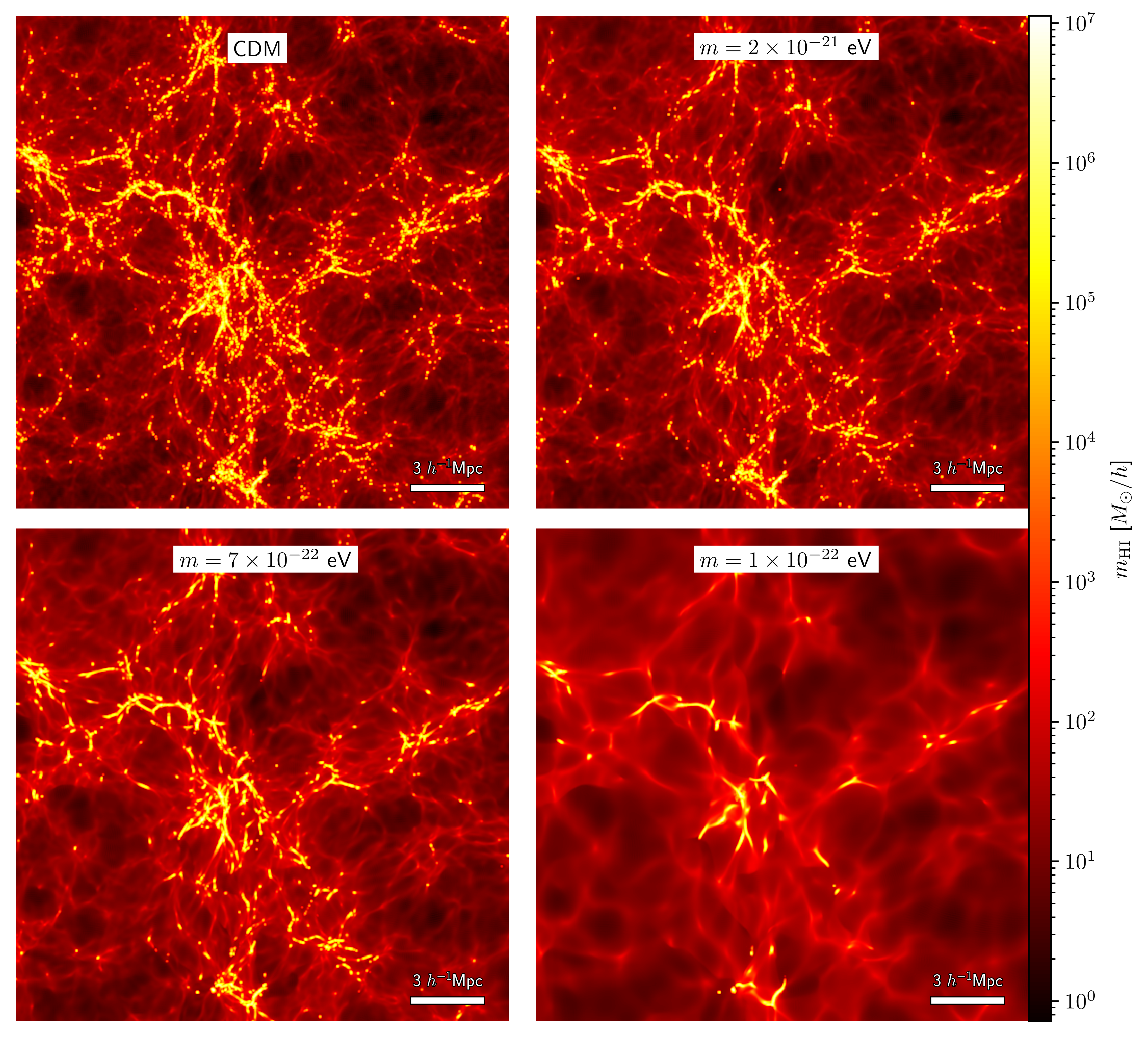
Fig. 2 shows some sigmoid-normalized \(64\times 64\) HI training maps in the top four rows across the CDM and cFDM cosmologies at \(z=4.94\). The bottom four rows show generated HIGlow HI samples with identical seeds across the cosmologies. There are no diverging pixels or other visual anomalies. Without the rescaled sigmoid in the conditional affine coupling layer, an alternative approach would have been to apply image clipping, constraining pixel values to fall within predefined maximum and minimum ranges, after each of the six flow blocks in the generative reverse flow. However, this would have come at the cost of losing important image features with each subsequent clipping operation.

The samples visually have very similar features compared to the input training data. The model has learned the effect of changing the axion mass \(m\) on the HI maps, and the characteristic suppression of small-scale structure at lower axion mass is apparent. We also show HIGlow samples for a synthetic cosmology corresponding to a new axion mass \(m=3\times 10^{-22}\) eV. The generated samples display subtle small-scale features that occupy an intermediate position between those of the \(m=10^{-22}\) eV and \(m=7\times 10^{-22}\) eV samples, aligning with our expectations. We have conducted comprehensive validation tests, the results of which are outlined in the following.

Fig. 2: Simulated data training samples (top four rows) and generated samples with HIGlow (bottom four rows) in the various cosmologies at \(z=4.94\). The \(64^2\) maps are \(2.5 \ h^{-1}\)Mpc a side. We add HIGlow samples for a conditional axion mass \(m = 3\times 10^{-22}\) eV. This case does not have corresponding simulation data, illustrated by crosses. The axion mass \(m\) decreases from right to left, with increased small-scale suppression.

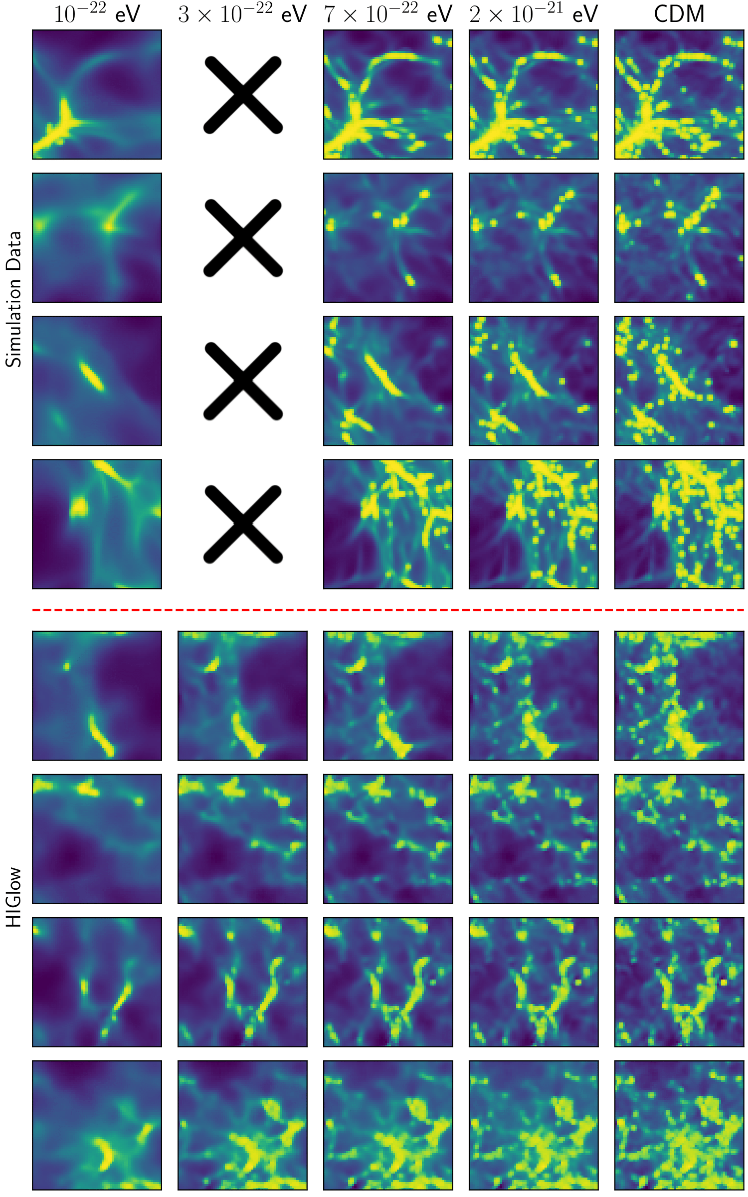
To ensure that the statistics of the generated HI maps follow the statistics of the simulation data, we use two validation metrics: HI mass PDFs and HI power spectra. Fig. 3 shows the HI mass PDFs as well as the mean power spectrum and the standard deviation for \(1000\) simulation data subcube projections (dotted lines) and the same number of HIGlow-generated samples (solid lines). The HI mass PDFs of the generated samples closely follow the target distribution, especially for HI masses below \(m_{\text{HI}} \approx 10^{5} \ M_{\odot}/h\). In the range \(m_{\text{HI}} = 10^5-10^7 \ M_{\odot}/h\), HIGlow captures the distribution less accurately, which is a result of the rarity of such high-mass pixels. For instance, \(m_{\text{HI}} = 10^6 \ M_{\odot}/h\) pixels are \(6-7\) orders of magnitude less likely than pixels with \(m_{\text{HI,peak}} \approx 20 \ M_{\odot}/h\). The PDF bump around this peak value broadly corresponds to the Ly\(\alpha\) forest in the post-reionization era (Zamudio et al. 2019).

Recall that we sigmoid-normalise the data before training HIGlow. The power spectra of Fig. 3 are also shown in sigmoid space since the trends with axion mass $m$ are more clear. We find that the target power spectra are reproduced with high fidelity, in particular the mean and standard deviation. The sigmoid-normalized power spectra exhibit the opposite trend with axion mass compared to the 3D non-sigmoid-normalized power spectra, see e.g. Carucci et al. (2015). We have checked and find that while the projection effect reduces the relative difference between cosmologies as reflected in 2D vs 3D power spectra, the sigmoid normalization reverses the trend.

In the evaluation of HIGlow, a conditional generative model, testing its capability to generate diverse samples spanning the entire latent space of axion masses is crucial. We test this functionality by choosing a new axion mass of \(m = 3\times 10^{-22}\) eV, unexplored by the simulations, and generating \(1000\) random images with HIGlow (see Fig. 2). Note that (unlike for CDM and the other three axion masses) we only show the HIGlow generated data for \(m = 3\times 10^{-22}\) eV, as the corresponding simulation data does not exist for this mass. The statistics of the synthetic cosmology are shown in Fig. 3, exhibiting a striking resemblance to the anticipated outcome. Falling in between the curves corresponding to \(m = 10^{-22}\) eV and \(m = 7 \times 10^{-22}\) eV, the generated distribution effectively showcases the interpolation prowess in latent space. While a direct comparison to actual simulations at \(m = 3 \times 10^{-22}\) eV would be needed for a more definitive test, the achieved success can be attributed to the monotonic albeit nonlinear influence of the axion mass \(m\) on the distribution of HI.

Fig. 3: Statistical properties of simulation data (dotted lines) and HIGlow-generated HI samples (solid lines) at \(z=4.94\) in CDM and cFDM cosmologies. We show HI mass PDFs (top panel), the median of 2D power spectra among \(1000\) random samples (middle panel) and their standard deviation (bottom panel). In cyan, we add the results for a conditional axion mass of \(m = 3\times 10^{-22}\) eV (see Fig. 2). This case does not have corresponding simulation data. The Nyquist frequency \(k_{\text{Ny}} = \pi N^{1/3} / L_{\text{box}}\) is shown as a vertical line.

Overall HI Abundance

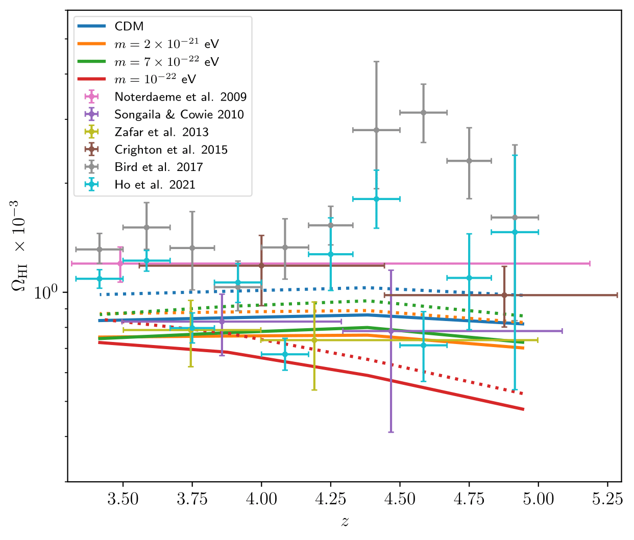
Here we investigate the overall HI abundance \(\Omega_{\text{HI}} = \bar{\rho}_{\text{HI}}(z)/\rho_{\mathrm{crit}}^0\) relative to the critical density of the Universe today \(\rho_{\mathrm{crit}}^0\), with \(\bar{\rho}_{\text{HI}}(z)\) being the mean HI density at redshift \(z\). Direct measurements from HIPASS (Barnes et al. 2001) and ALFALFA (Oman 2022) have been used to detect individual extra-galactic objects, allowing constraints on the HI mass function and abundance of low redshift (\(z\approx 0\)) HI at around \(\Omega_{\mathrm{HI}} \sim (3.9 \pm 0.6) \times 10^{-4}\). At slightly higher redshift, cross-correlations with optical tracers (e.g. DEEP2 or WiggleZ) lead to estimates of the HI abundance at \(z\sim 0.8\) to be \(\Omega_{\mathrm{HI}}b_{\mathrm{HI}} \sim 6.2^{+2.3}_{-1.5} \times 10^{-4}\) (Switzer et al. 2013). More indirect measurements of DLAs allow us to constrain the HI abundance up to \(z\sim 5\). Therefore, in the post-reionization era, we have a well-defined target for the amplitude of the 21 cm signal, which is proportional to the square of the HI abundance, \(P_{21} \propto \Omega_{\text{HI}}^2\).

We show the value of \(\Omega_{\text{HI}}(z)\) in the four simulated cosmologies in Fig. 4 in the redshift range \(z=3.42-4.94\). To compare our predictions to observations, we first note that in a typical DLA survey, HI column densities are estimated from absorption spectra of quasars. The HI frequency distribution or column density distribution function (CDDF) is typically written as

\[f_{\text{HI}}(N_{\text{HI}}, X) = \frac{\mathrm{d}^2N(N_{\text{HI}})}{\mathrm{d}N_{\text{HI}}\mathrm{d}X},\]

where \(N\) is the number of lines of sight with column densities between \(N_{\text{HI}}\) and \(N_{\text{HI}}+\mathrm{N_{\text{HI}}}\), and

\[\mathrm{d}X = \frac{H_0}{H(z)}(1+z)^2\mathrm{d}z\]

is the so-called absorption distance. The absorption distance has the property that absorbers with non-evolving number density \(n_a\) and cross-section \(\sigma_a\) (both in proper length units) will produce a constant number of absorption lines per unit absorption distance, i.e. \(\mathrm{d}N/\mathrm{d}X = \text{const}\). The distribution \(f_{\text{HI}}(N_{\text{HI}}, X)\) spans ten orders of magnitude from around \(N_{\text{HI}}=10^{12}\) cm\(^{-2}\), below which Ly\(\alpha\) absorbers produce absorption lines too weak to be recognized, to \(10^{22}\) cm\(^{-2}\) above which absorbers are very rare. Quasar absorbers with HI column densities below \(\simeq 10^{17.3}\) cm\(^{-2}\) are called the Ly\(\alpha\) forest, and physically represent the low-density and highly ionized gas that resides in the IGM. Systems with column densities above \(N_{\text{HI,DLA}}=10^{20.3}\) cm\(^{-2}\) are called DLAs, which typically correspond to extra-galactic regions and are self-shielded against external radiation. Systems with column densities in between these two regimes, are called Lyman Limit Systems (LLSs) in the range \(10^{17.3}-10^{19.0}\) cm\(^{-2}\) and sub-DLAs in the range \(10^{19.0}-10^{20.3}\) cm\(^{-2}\). The DLAs account for most of the HI, but it is the Ly\(\alpha\) forest that accounts for most of the gas (neutral + ionized).

The total gas density can be inferred from the HI CDDF via

\[\Omega_{\mathrm{g}}^{\mathrm{DLA}}(X)\mathrm{d}X = \frac{\mu m_{\mathrm{p}}H_0}{c\rho_{\mathrm{crit}}^0}\int_{10^{20.3}}^{\infty}N_{\mathrm{HI}}f_{\mathrm{HI}}(N_{\mathrm{HI}}, X)\mathrm{d}X,\]

where \(\mu = 1.3\) is the mean molecular mass of the gas. In the discrete limit, \(\Omega_{\mathrm{g}}^{\mathrm{DLA}}\) is given by

\[\Omega_{\mathrm{g}}^{\mathrm{DLA}} = \frac{\mu m_{\mathrm{p}}H_0}{c\rho_{\mathrm{crit}}^0}\frac{\sum N_{\mathrm{HI}}}{\Delta X},\]

where the sum is calculated for systems with \(\log_{10}N_{\mathrm{HI}}\geq 20.3\) along lines of sight with a total pathlength of \(\Delta X\). As noted in (Crighton et al. 2015), we can convert the gas mass in DLAs \(\Omega_{\mathrm{g}}^{\mathrm{DLA}}\) to the neutral hydrogen mass via

\[\Omega_{\mathrm{HI}} = \delta_{\mathrm{HI}}\Omega_{\mathrm{g}}^{\mathrm{DLA}}/\mu,\]

where \(\mu\) accounts for the mass of helium and \(\delta_{\mathrm{HI}}=1.2\) estimates the contribution from systems below the DLA threshold of \(10^{20.3}\) cm\(^{-2}\). In Fig. 4, we add a compilation of measurements, each accompanied by error bars, sourced from multiple studies. Note that all the estimates have been corrected for helium content and cosmological factors. Specifically, both the Hubble constant \(H_0\) and the absorption distance \(\Delta X\) in the CDDF equation have been accounted for.

Within the error bars, the agreement between the results from simulations and observations is good. Hydrodynamic simulations like ours using the TNG galaxy formation module typically agree better with observations than semi-analytic models (Lagos et al. 2014) and are comparable to the agreement found using the EAGLE simulations (Rahmati et al. 2015). The trend of decreasing HI abundance towards smaller axion mass \(m\) agrees well with the WDM results of Carucci et al. (2015). The thermal relic WDM masses explored in Carucci et al. (2015) correspond to axion masses of \(m\in [1.6\times 10^{-22},5.5\times 10^{-21}]\) eV.

We note that similar to Villaescusa-Navarro et al. (2018), the overall HI abundance depends on resolution. The lower-resolution \(N=512^3\) simulations contain \(\sim 10\)% less HI in the explored redshift interval \(z=3.42-4.94\) than the higher-resolution \(N=1024^3\) runs shown in Fig. 4. HI can reside in small halos of mass \(M_h \sim 10^9 \ M_{\odot}/h\), few of which are resolved by the \(N=512^3\) runs. For halo-based HI estimations such as those based on the halo model (Villaescusa-Navarro et al. 2018), the trend with changing resolution is most intuitive, but it is also reproduced in particle-based models as we find.

Fig. 4: Comparison of mock and observed cosmic HI density estimates. The abundance parameter \(\Omega_{\text{HI}}=\bar{\rho}_{\text{HI}}(z)/\rho_c^0\) from simulations in the redshift range \(z=3.42-4.94\) for various cosmologies is shown by dotted lines (in real space) and solid lines (in redshift space), obtained using the procedure outlined in Dome et al. (2023). Observational measurements are displayed with \(1\sigma\) error bars: Songaila & Cowie (2010) provide DLA measurements from Keck data; Zafar et al. (2013) quote combined DLA and sub-DLA measurements from ESO UVES; Crighton et al. (2015) quote results from a Gemini GMOS study of DLAs; Noterdaeme et al. (2009), Bird et al. (2017) and Ho et al. (2021) are DLA analyses using SDSS DR7, DR12 and DR16Q, respectively.

HI Power Spectrum and Bias

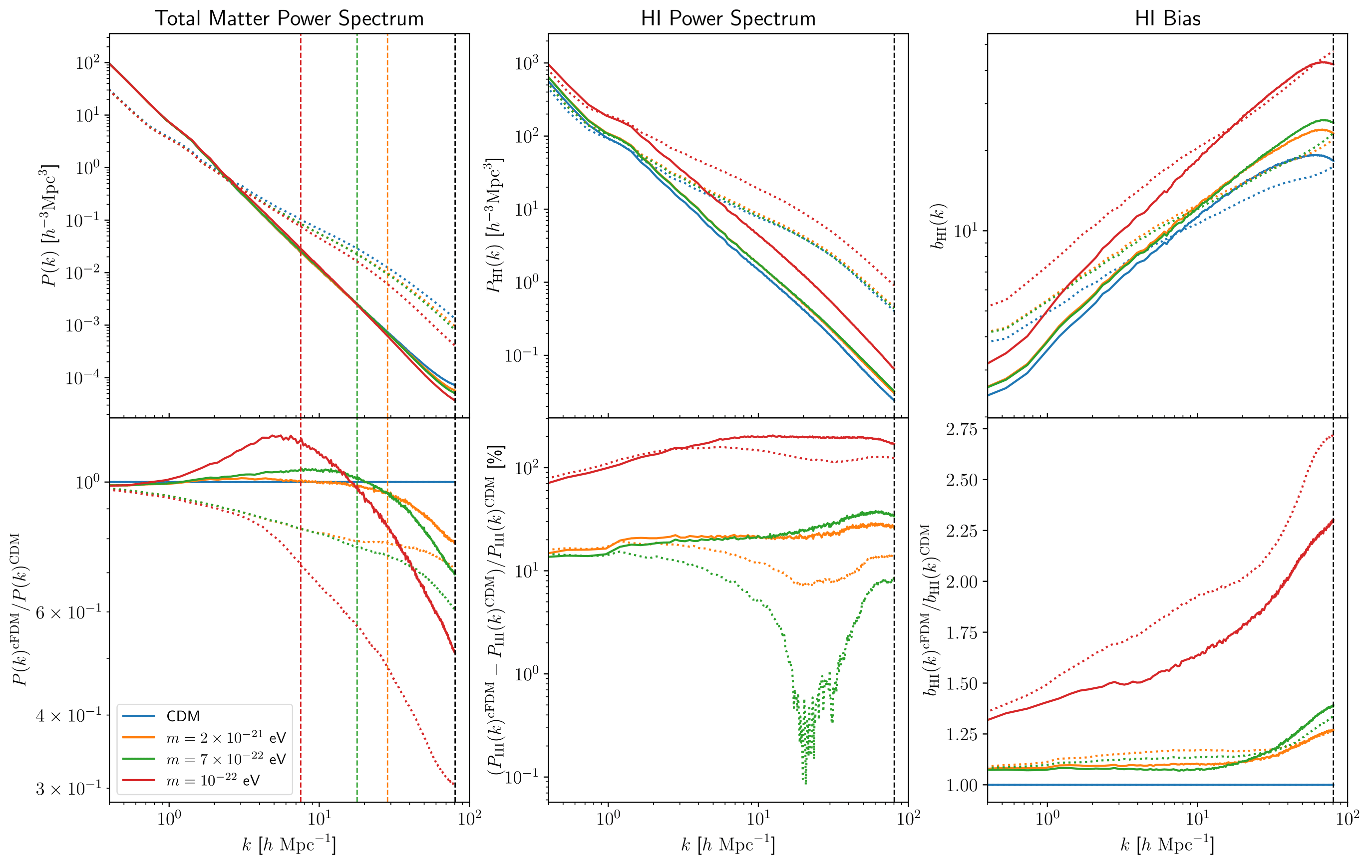
In Fig. 5, we show the total matter and HI power spectrum estimated using a third-order piecewise cubic spline (PCS) mass-assignment scheme and subsequent Fourier transformation,

\[P_{X} = \frac{1}{N_{\text{modes}}}\sum_{\mathbf{k}\in k}\delta_{X}(\mathbf{k})\delta_{X}^{\ast}(\mathbf{k}),\]

with \(X = \lbrace \text{tot}, \text{HI}\rbrace\) and \(N_{\text{modes}}\) being the number of modes lying in the spherical shell \(k\) of width \(\delta k = 2\pi / L_{\text{box}}\). When calculating the HI power spectrum, we do not account for the fact that the actual density profile of the gas particles is not given by a uniform cube but described by the SPH kernel. A reliable amplitude mode correction implementation is beyond the scope of this paper, also see Villaescusa-Navarro et al. (2014). However, we compensate for the MAS window function to improve the power spectrum fidelity on scales close to the Nyquist frequency \(k_{\text{Ny}} = \pi N^{1/3} / L_{\text{box}}\), where \(N^{1/3}\) is the number of cells per box side.

Fig. 5: Total matter (left panel), HI power spectrum (middle panel) and HI bias (right panel) in CDM and cFDM cosmologies at \(z=4.94\). Each panel shows results in real space (dotted lines) and redshift space (solid lines). The vertical dashed lines mark the cFDM half-mode scale \(k_{1/2}\) (colored) as per Marsh (2016) and the Nyquist frequency \(k_{\text{Ny}} = \pi N^{1/3} / L_{\text{box}}\) (in black). In the bottom row, we present the ratio of results between cFDM and CDM, with the first and third panels displaying the absolute ratio and the second panel showing the relative difference in percent. Both HI clustering and HI bias \(b_{\text{HI}}^2(k) = P_{\text{HI}}(k)/P_{\text{tot}}(k)\) increase for decreasing axion mass \(m\).

In cFDM cosmologies, the total matter power spectrum in Fig. 5 follows the well-known trend of small-scale suppression for wavenumbers above \(k_{1/2}\) (Marsh 2016). The effect of peculiar velocities, also called redshift-space distortions (RSDs), can be clearly discerned. On large scales, the clustering of matter in redshift space is enhanced due to the Kaiser effect (Kaiser 1987). On small scales, the peculiar velocities, particularly inside halos, give rise to the Fingers of God, suppressing the amplitude of the total matter power spectrum (Tegmark et al. 2004).

HI is more clustered than the total matter since the UV background ionizes hydrogen in environments that are not dense enough to self-shield. As opposed to the suppression beyond \(k_{1/2}\) in the total matter clustering, the HI power spectrum does not exhibit a small-scale cut-off since most of the HI is trapped in intermediate- and high-mass halos. Contrary to a naive expectation, HI clustering increases with decreasing axion mass \(m\). Since most of the HI is locked inside DM halos in the post-reionization era, the higher halo bias in cFDM cosmologies compared to CDM (Dunstan et al. 2011) leads to an increased HI clustering. This is in agreement with Carucci et al. (2015) who showed that the amount of HI per total mass in a given DM halo mass bin is very similar between CDM and WDM cosmologies for particle-based HI modeling approaches. As a result, the spatial distribution of HI is more biased in the cFDM models than in CDM, with the bias increasing with decreasing axion mass \(m\). In the extreme cFDM model with \(m=10^{-22}\) eV, deviations from CDM in the HI power spectrum can reach more than \(300\)% at \(z=4.94\), in agreement with WDM results from Carucci et al. (2015).

The HI bias

\[b_{\text{HI}}(k) = \sqrt{\frac{P_{\text{HI}}(k)}{P_{\text{tot}}(k)}}\]

describes the bias between the distributions of HI and the total matter. While the HI bias defined using the above equation suffers from stochasticity (shot noise), it is closer to observations than results inferred using the alternative definition involving the HI-matter cross-correlation, \(b_{\text{HI}}(k) = P_{\text{HI-tot}}(k)/P_{\text{tot}}(k)\) (Castorina & Villaescusa-Navarro 2017). As shown in Fig. 5, the large-scale halo bias in CDM at \(z=4.94\) attains values \(b_{\text{HI}} \approx 2.5\) in redshift space and \(b_{\text{HI}} \approx 3.5\) in real space, in agreement with previous work (Wang et al. 2021). On the smallest (strongly non-linear) scales probed, it increases up to \(b_{\text{HI}} \approx 20\). In cFDM cosmologies, the HI bias increases with decreasing axion mass $m$, and for the extreme \(m=10^{-22}\) eV model, the bias ratio between cFDM and CDM can reach values above \(\approx 2.5\).

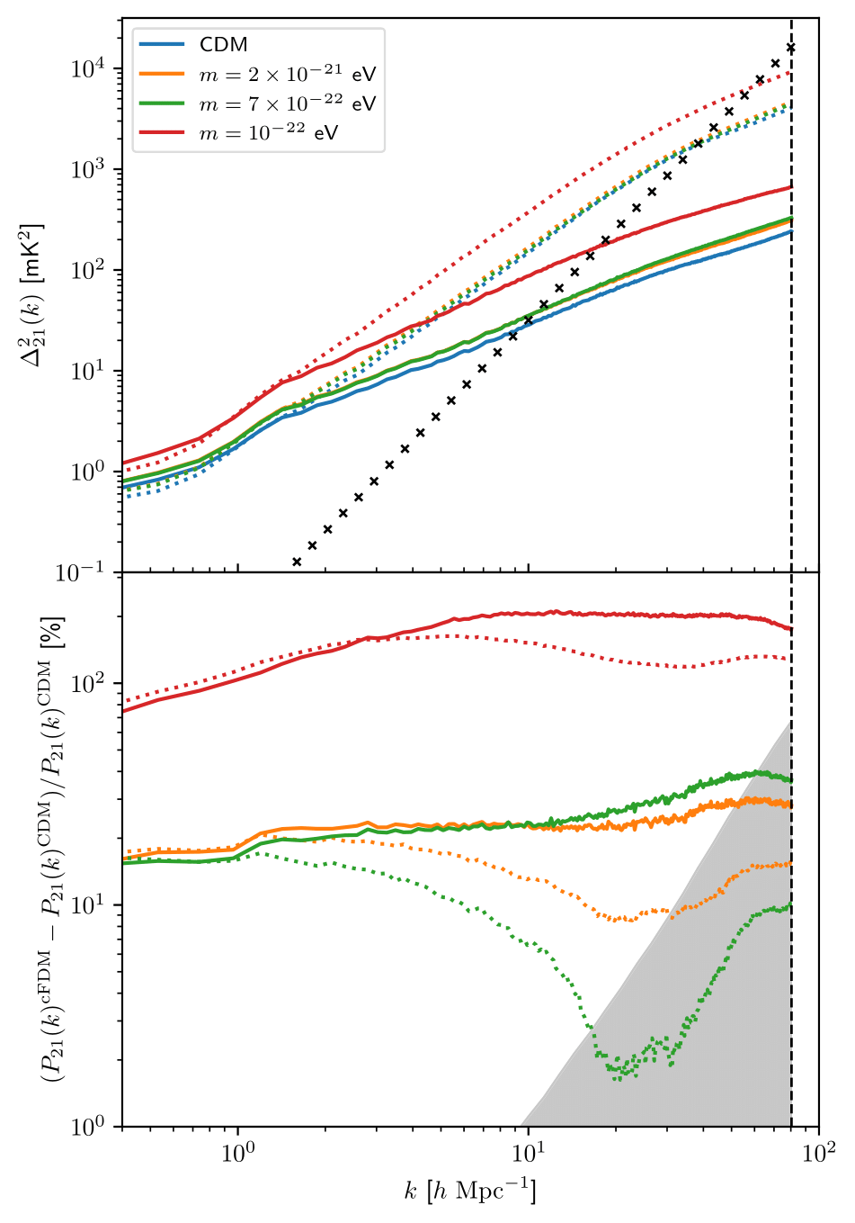
The clustering of the 21 cm signal is shown in Fig. 6. Its magnitude \(\propto \Omega_{\text{HI}}^2(z)\) in the post-reionization era is several orders of magnitude lower than before and during reionization, and exhibits a clear trend with decreasing axion mass \(m\). The SKA1-Low system noise is shown for instrument parameters from Table 1, assuming an optimistic foreground wedge model in which all \(k\) modes inside the primary field of view are excluded (Pober et al. 2014). Note that we exclude the error arising from sample variance, which predominantly affects larger scales. We find that at \(z=4.94\), the 21 cm power spectrum will be detected by this telescope up to scales \(k\approx 9\) \(h\)/Mpc in CDM and the less extreme cFDM models \(m\sim 10^{-21}\) eV, while it can be detected up to \(k\approx 15\) \(h\)/Mpc in the more extreme \(m=10^{-22}\) eV model.

Since we assume that \(T_\gamma/T_s \approx 0\) in our modeling, the relative difference in the 21 cm power spectrum between cFDM and CDM is identical to the relative difference in the HI power spectrum shown in Fig. 5. We also show the normalized error \(\Delta^2_{\text{noise}}/\Delta^2_{21,\text{CDM}}\) for SKA1-Low, representing the \(1\sigma\) system noise error on the 21 cm dimensionless power spectrum of the model with CDM. While the more extreme \(m=10^{-22}\) eV model can be distinguished from CDM at the \(2\sigma\) confidence level across all scales (\(k< 80 \ h/\)Mpc) resolved by the simulations, SKA1-Low will not be able to discriminate among CDM and the less extreme cFDM models \(m\sim 10^{-21}\) eV with \(1080\) hours of observations on small scales \(k\approx 70\) \(h\)/Mpc.

Fig. 6: 21 cm power spectrum in CDM and cFDM cosmologies at \(z=4.94\). We show results for the “dimensionless” power spectrum \(\Delta^2_{21}(k)=k^3P_{21}(k)/(2\pi^2)\), in both real space (dotted lines) and redshift space (solid lines). Black crosses denote the expected SKA1-Low \(1\sigma\) system temperature noise \(\Delta^2_{\text{noise}}\) for \(1080\) hours of observation in a \(8\) MHz bandwidth with \(290\) frequency channels as per Table 1, for an optimistic foreground wedge model. The vertical dashed line denotes the Nyquist frequency \(k_{\text{Ny}} = \pi N^{1/3} / L_{\text{box}}\) (in black). In the bottom panel, we present the relative difference between cFDM and CDM, identical to the relative difference in the HI power spectrum, see Fig. 5. The normalized error \(\Delta^2_{\text{noise}}/\Delta^2_{21,\text{CDM}}\) on the CDM 21 cm power spectrum for the same instrument parameters in SKA1-Low is shown by a shaded region. 21 cm clustering increases for decreasing axion mass \(m\).

HI Column Density Distributions

Another quantity commonly employed to study the distribution of HI in the post-reionization era is the HI CDDF. As mentioned, HI column densities of Ly\(\alpha\) clouds, LSS, sub-DLAs and DLAs are inferred observationally from quasar spectra.

To compare mock HI CDDFs to observational datasets, we first assign the HI to gas particles. Then, the value of the column density \(N_{\text{HI}}\) along an arbitrary line of sight (LOS) can be computed following a method from Villaescusa-Navarro et al. (2014) which we briefly summarize here. We first project all the gas particle positions onto the XY Cartesian plane, draw LOSs on a regular grid perpendicular to the XY plane from \(Z=0\) to \(Z=L_{\text{box}}\). For a given LOS, if the minimum distance between any gas particle \(i\) and the LOS (i.e. impact parameter \(b_i\)) is smaller than the smoothing length \(h_i\) of the gas particle, then we pick up a contribution based on the integrated density along the path that the LOS intersects the physical size of the gas particle:

\[N_{\text{HI},i} = 2\frac{m_{\text{HI}}}{m_{\text{H}}}\int_0^{l_{\text{max}}}W(r,h_i)\mathrm{d}l,\]

where \(N_{\text{HI},i}\) is the column density due to particle \(i\), having HI mass \(m_{\text{HI}}\) and SPH smoothing length \(h_i\) while \(m_{\text{H}}\) is the mass of the hydrogen atom. The relation between the radius \(r\) and the integration variable \(l\) is given by \(r^2=b^2+l^2\), with \(l_{\text{max}}^2=h_i^2-b^2\). Our regular grid consists of \(10,000 \times 10,000\) points, i.e. the number of LOSs is \(10^8\). In view of our small box size \(L_{\text{box}} = 40 \ h^{-1}\)Mpc, the probability of encountering more than a single absorber with a large column density \(\sim 10^{19}\) cm\(^{-2}\) along the LOS is negligible. Our results are thus converged for sub-DLAs and DLAs for which we can, as a result, safely ignore light-cone effects. We repeated the tests mentioned in Villaescusa-Navarro et al. (2014) to verify that the grid is fine enough to achieve convergence. For instance, when slicing the box into slabs of different widths and computing the column densities from any of those slabs, the frequency distribution does not change above \(\sim 10^{19}\) cm\(^{-2}\).

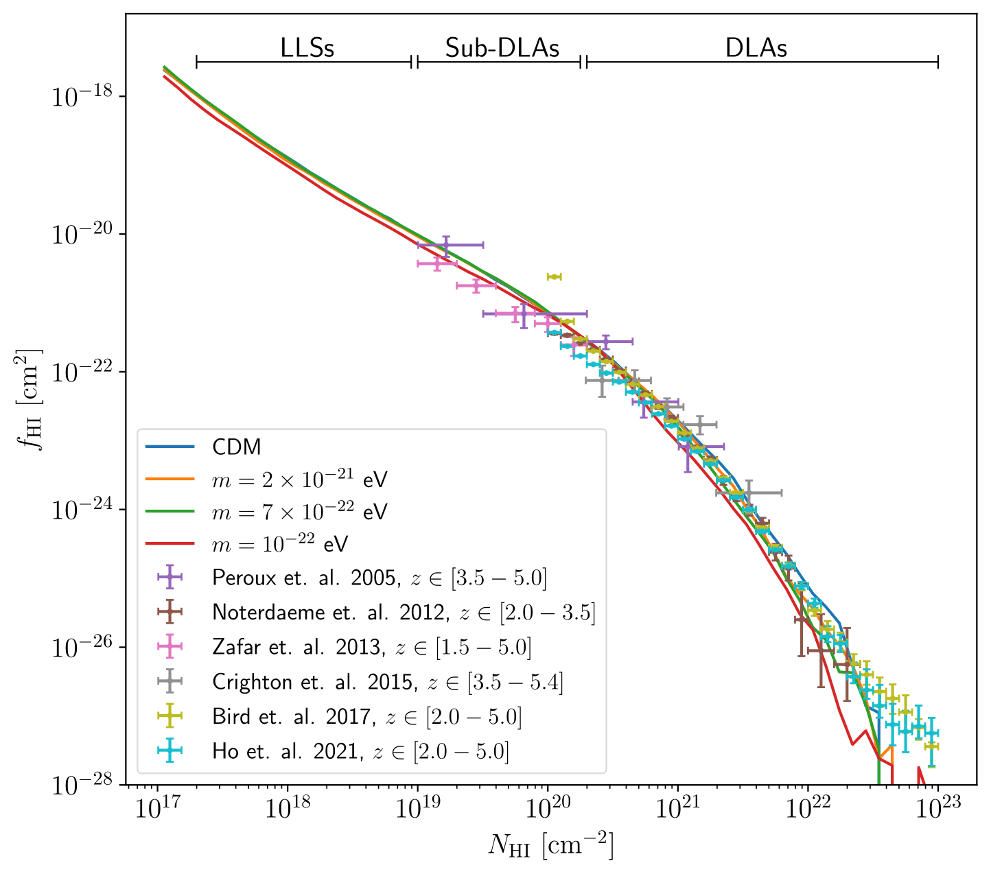
The inferred frequency distribution of HI column densities in CDM and cFDM cosmologies is shown in Fig. 7. We assume a weak redshift dependence of the HI column distribution in the range \(z=2-4\), which can be understood in the modeling framework of Theuns (2021) based on cosmological accretion of gas onto DM halos. Hence, we can overlay results from observations at redshifts \(z=[1.5-4.0]\). Since the (sub-)DLAs at \(z>4\) are rare and typically inferred from noisy spectra, they mostly contribute to enlarged error bars and we can extend the redshift range to \(z=[1.5-5.0]\). We thus add various measurements with errorbars to Fig. 7. As shown in the most recent measurement paper (Ho et al. 2021), the trend beyond \(z>4\) is in fact still unclear due to statistical uncertainties in the measurements. To better align with the observations, the results in the CDM and cFDM models are shown at \(z=3.42\) rather than \(z=4.94\) as for the bulk of this paper.

For CDM and the less extreme cFDM models \(m=7\times 10^{-22}\) eV and \(m=2\times 10^{-21}\) eV, we find good agreement with the observations. The strongest DLA absorbers are not modeled well in any of the simulated cosmologies, which can be traced to our moderate box size of \(L_{\text{box}} = 40 \ h^{-1}\)Mpc. The more extreme \(m=10^{-22}\) eV model is visually at odds with the measurements since the predicted CDDF undercuts observational estimates for column densities above \(N_{\text{HI}} = 2\times 10^{21}\) cm\(^{-2}\). With larger data sets and better mean flux measurements, one might be able to put competitive astrophysical constraints on FDM models.

Fig. 7: Column density distribution function of HI absorbers. Results at \(z=3.42\) in CDM and cFDM cosmologies are traced by solid lines. Data from observations are shown with \(1\sigma\) error bars: Peroux et al. (2005) quote (sub-)DLA measurements from ESO UVES; Noterdaeme et al. (2012) perform a DLA analysis using SDSS DR9 data; Zafar et al. (2013) quote sub-DLA measurements from ESO UVES; Crighton et al. (2015) quote results from a Gemini GMOS study of DLAs; Bird et al. (2017) and Ho et al. (2021) perform a DLA analysis using SDSS DR12 and DR16Q data, respectively. The redshift ranges in the legend refer to the (sub-)DLA redshifts and not the emission redshifts of the quasars.

DLA Cross-Sections

Next, we focus on absorbers with high column densities above \(N_{\text{HI,DLA}}=10^{20.3}\) cm\(^{-2}\), i.e. DLAs and their cross-sections. The latter are of interest since the observed rate of incidence of DLAs tells us the product of the number density of DLAs times their cross-section (Pérez-Ràfols et al. 2018). Both the number density and the cross-section of absorbers is expected to be sensitive to DM physics. In cFDM cosmologies, the high column density of cosmic filaments at \(z=2-5\) (Gao et al. 2015) should be reflected in the cross-section distribution, which we now investigate for the first time.

We compute the DLA cross-section as follows. For each DM halo, we select the gas particles belonging to the halo and we throw random LOSs within the halo virial radius. After computing the column density for each LOS, the DLA cross-section is readily obtained as

\[\sigma_{\text{DLA}} = \pi R_{\text{vir}}^2\left(\frac{n_{\text{DLA}}}{n_{\text{tot}}}\right),\]

where \(R_{\text{vir}}\) is the halo virial radius, \(n_{\text{DLA}}\) is the number of LOSs with column density above \(10^{20.3}\) cm\(^{-2}\) and \(n_{\text{tot}}\) is the total number of LOSs used. The virial radius is determined as per the Bryan & Norman (1998) spherical collapse result, but we checked that our results do not change if we use a different definition for \(R_{\text{vir}}\). We use \(40,000\) random LOSs for each DM halo, and find that our results do not change significantly when we increase the number.

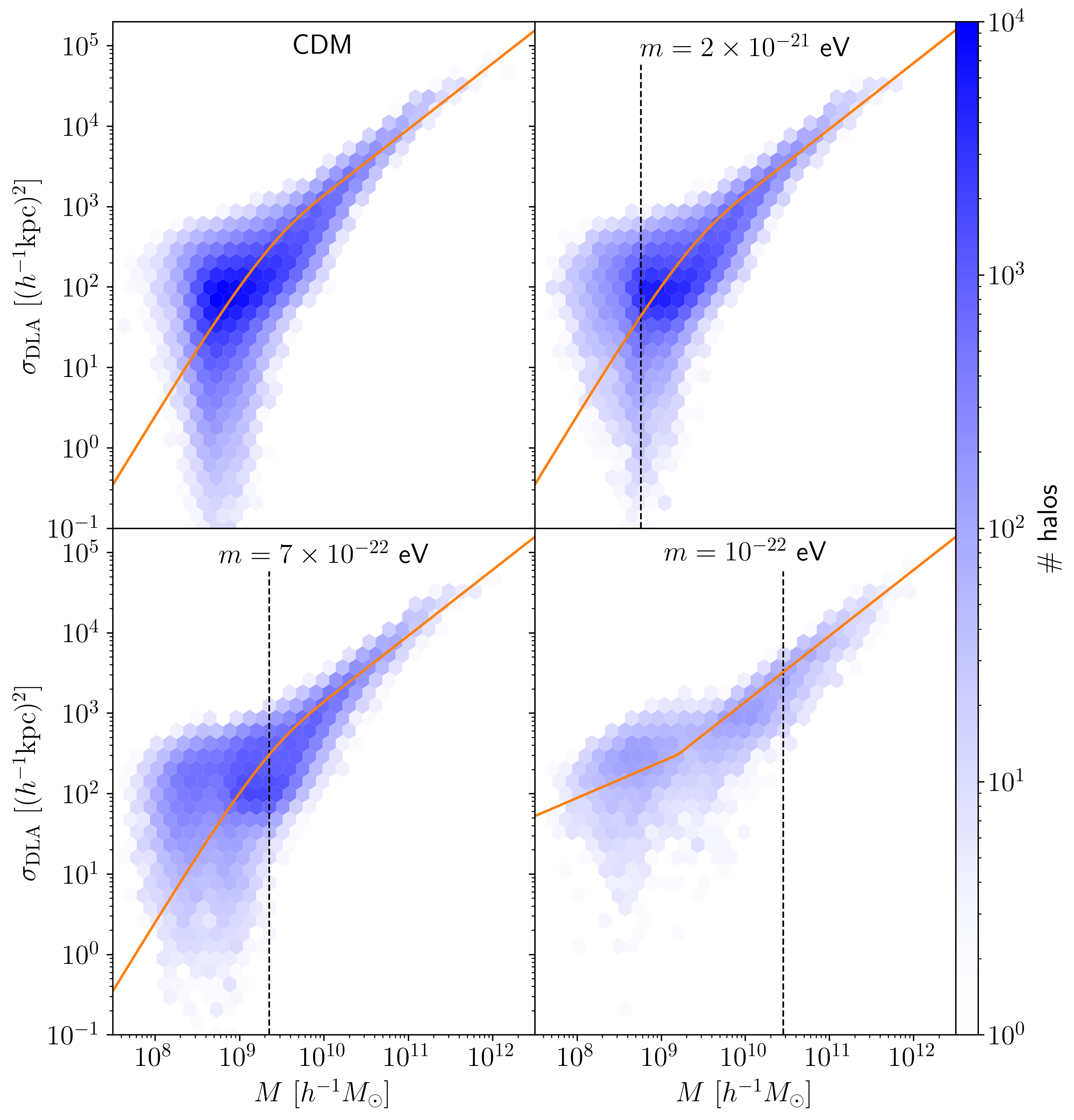
We show results in Fig. 8. We find that the mean DLA cross-section increases with halo mass, which apart from the \(m=10^{-22}\) eV cosmology is well fitted by the following function

\[\sigma(M | N_{\text{HI,DLA}},z)=A\left(\frac{M}{h^{-1}M_{\odot}}\right)^{\alpha}\left(1-e^{-(M/M_0)^{\beta}}\right).\]

In agreement with the CDM analysis of Villaescusa-Navarro et al. (2018), we find that the slope of the cross-section for large halo masses has best-fit value \(\alpha = 0.82\) and the characteristic halo mass where the DLA cross-section decreases exponentially has a strong correlation with the overall normalization of the function, \(A\cdot M_0 = 14100 \ h^{-3}\text{kpc}^2M_{\odot}\). The cutoff exponent is well approximated by \(\beta = 0.85 \cdot \log_{10}(N_{\text{HI,DLA}}/\text{cm}^{-2})-16.35\), the only redshift dependence remaining in \(M_0\) and \(A\). At \(z=4.94\) which is shown in Fig. 8, the characteristic halo mass is \(M_0 = 1.6\times 10^9 \ h^{-1}M_{\odot}\) in all three cosmologies. In Table 2, we present best-fit values for \(M_0\) across redshifts \(z=3.42-4.94\), which decreases with redshift implying that less massive halos can host HI at higher redshift, also see Villaescusa-Navarro et al. (2018).

Configuration
Array design	512 compact core
Station diameter \(D\) [m]	35
Integration time \(t_{\mathrm{int}}\) [s]	60
Bandwidth \(B\) [MHz]	8
Number of channels \(N_{\text{chan}}\)	29/290
Frequency resolution \(\Delta \nu\) [kHz]	272
Number of observing hours/days	6/180
Redshift/frequency [MHz]	4.94/238.9
Angular resolution \(\theta_{\mathrm{A}}\)	0.5’, 1’, 2’
Primary beam’s FWHM \(\theta_{\mathrm{max}}\)	3.12(\(\nu/200\) MHz)\(^{-1}\) deg
Single baseline noise error \(\sqrt{\langle N^2\rangle}\) [Jy]/[mK]	0.55/134

Table 1: Summary of SKA1-Low instrument parameters used in this study to obtain the thermal noise sensitivity. The FWHM of the primary beam agrees well with Kakiichi et al. (2017) and Hassan et al. 2020. Natural sensitivities \(A_{\mathrm{eff}}/T_{\mathrm{sys}}\) as a function of frequency are tabulated in Braun et al. (2019).

While a small secondary peak emerges in the cross-section distribution for the \(m=7\times 10^{-22}\) eV model, the \(m=10^{-22}\) eV cosmology exhibits a bimodal distribution at \(z=4.94\). The median cross-section is significantly higher than in the other three cosmologies for halo masses below \(M\approx 3\times 10^9 \ M_{\odot}/h\), which is about an order of magnitude below the half-mode mass \(M_{1/2}\) (Marsh 2016). We thus confirm the prediction of (Gao et al. 2015) that the high column density of cosmic filaments in cFDM/WDM cosmologies is reflected in the properties of DLAs. This is also in agreement with cosmic web studies at high redshift, which show that the mean DM overdensity in filaments at \(z\approx 5\) is around \(30\)% higher in the \(m=10^{-22}\) eV cosmology than for CDM (Dome et al. 2022). The power law + cutoff parametrization thus gives a poor fit for the \(m=10^{-22}\) eV model, and instead we adopt a double power law

\[\sigma(M | N_{\text{HI,DLA}},z)= \begin{cases} & A\left(\frac{M}{h^{-1}M_{\odot}}\right)^{\alpha} \ \ \text{if} \ \ M > M_{\mathrm{break}} \\ & B\left(\frac{M}{h^{-1}M_{\odot}}\right)^{\beta} \ \ \text{else}. \end{cases}\]

The dependence of \(\sigma_{\mathrm{DLA}}\) on cosmology at the high-mass end (i.e. \(M > M_{\mathrm{break}}\)) is so weak that the normalization \(A\) can still be well approximated by \(A\cdot M_0 = 14100 \ h^{-3}\text{kpc}^2M_{\odot}\), where \(M_0\) is taken from the power law + cutoff parametrization. The normalization at the low-mass end \(B\) is determined by ensuring that the two power laws intersect at \(M_{\mathrm{break}}\). We provide the best-fit values for \(M_{\mathrm{break}}\) and \(\beta\) in Table 2.

	\(M_0 \ [M_{\odot}/h]\)	\(M_{\mathrm{break}} \ [M_{\odot}/h]\)	\(\beta\)
\(z=3.42\)	\(3.6\times 10^9\)	\(1.5\times 10^9\)	\(0.52\)
\(z=3.88\)	\(2.6\times 10^9\)	\(1.6\times 10^9\)	\(0.51\)
\(z=4.38\)	\(1.9\times 10^9\)	\(1.7\times 10^9\)	\(0.48\)
\(z=4.94\)	\(1.6\times 10^9\)	\(1.6\times 10^9\)	\(0.45\)

Table 2: Best-fit parameters \(M_0\) in power law + cutoff parametrization for CDM, \(m=2\times 10^{-21}\) eV and \(m=7\times 10^{-22}\) eV cosmologies and \(M_{\mathrm{break}}\), \(\beta\) in the double power law parametrization for the \(m=10^{-22}\) eV cosmology across redshifts \(z=3.42-4.94\).

Using the mean DLA cross-section, we can estimate the DLA bias as

\[b_{\text{DLA}}(z|N_{\text{HI,DLA}}) =\frac{\int_0^{\infty}b(M,z)n(M,z)\sigma(M|N_{\text{HI,DLA}},z)\mathrm{d}M}{\int_0^{\infty}n(M,z)\sigma(M|N_{\text{HI,DLA}},z)\mathrm{d}M},\]

where \(n(M,z)\) denotes the halo mass function (HMF) and \(b(M,z)\) the halo bias. We take the HMF from Sheth & Tormen for CDM and apply the Schneider et al. (2012) rescaling for cFDM. For the halo bias, we use the fitting formula in Tinker et al. (2010), which expresses the bias \(b(M,z)\) as a function of the peak height \(\nu=\delta_c/\sigma(M)\), where \(\delta_c = 1.686\) is the spherical collapse threshold and \(\sigma^2(M)\) the linear matter variance. This parametrization provides a reliable fit for the bias of both CDM and cFDM halos when adopting the variance \(\sigma^2(M)\) in the respective cosmology (Dunstan et al. 2011).

In Table 3, we show the estimated values for the DLA bias in the various cosmologies across redshifts \(z=3.42-4.94\), for absorbers with column density \(N_{\text{HI}} > N_{\text{HI,DLA}} = 10^{20.3}\) cm\(^{-2}\). We find that the DLA bias increases with redshift at the explored post-reionization redshifts. Since the gas in the IGM is denser and the amplitude of the UV background decreases with redshift, this trend is expected for the DLA bias as well as the HI bias. Typically, both biases have similar magnitudes, \(b_{\text{DLA}} \simeq b_{\text{HI}}\), following the theoretical arguments in Castorina & Villaescusa-Navarro (2017) and comparing the values in Table 3 to the \(b_{\text{HI}}\) estimates from Fig. 5 at \(z=4.94\). In cFDM cosmologies, we find the redshift-independent trend that the DLA bias increases with decreasing axion mass \(m\), from \(b_{\text{DLA}} = 2.3\) for CDM to \(b_{\text{DLA}} = 3.8\) for the \(m=10^{-22}\) eV model at \(z=4.94\). This trend is primarily a result of the increased halo bias in cFDM cosmologies.

	\(\mathrm{CDM}\)	\(2\times 10^{-21} \ \mathrm{eV}\)	\(7\times 10^{-22} \ \mathrm{eV}\)	\(10^{-22} \ \mathrm{eV}\)
\(z=3.42\)	\(1.8\)	\(2.0\)	\(2.1\)	\(2.6\)
\(z=3.88\)	\(1.9\)	\(2.2\)	\(2.3\)	\(2.9\)
\(z=4.38\)	\(2.1\)	\(2.3\)	\(2.6\)	\(3.3\)
\(z=4.94\)	\(2.3\)	\(2.6\)	\(2.9\)	\(3.8\)

Table 3: DLA bias \(b_{\text{DLA}}\), in CDM and cFDM cosmologies across redshifts \(z=3.42-4.94\).

It is useful to compare our estimates of the DLA bias to observations. Through cross-correlating the DLAs with the Ly\(\alpha\) forest, (Pérez-Ràfols et al. 2018) measured a DLA bias factor of \(b_{\text{DLA}} = 1.99\pm 0.11\), while using cross-correlations with CMB lensing data Alonso et al. 2018 and Lin et al. 2020 measured \(b_{\text{DLA}} = 2.6\pm 0.9\) and \(b_{\text{DLA}} = 1.37^{+1.30}_{-0.92}\), respectively. All three estimates are for a median DLA redshift of \(z_{\mathrm{median}}=2.3\) and agree well with our CDM estimates from Table 3, if we assume a linear relationship from \(z=3.9\) to \(z=2.3\), e.g. Villaescusa-Navarro et al. (2018). With more powerful (combined) datasets and a better understanding of the theoretical systematics involved, the observed DLA bias could be used to put constraints on FDM-like cosmologies.

Fig. 8: DLA cross-section of halos at \(z=4.94\). The color of each hexbin is proportional to the number of halos. For the CDM (top left), \(m=2\times 10^{-21}\) eV (top right) and \(m=7\times 10^{-22}\) eV (bottom left) cosmologies, we fit a power law + exponential function while for the \(m=10^{-22}\) eV (bottom right) cosmology we fit a double power law. The vertical dashed line denotes the half-mode mass \(M_{1/2}\) (Marsh 2016). The small secondary peak in the \(m=7\times 10^{-22}\) eV model morphs into a bimodal distribution in the \(m=10^{-22}\) eV cosmology.

Mock Radio Maps For SKA-Low

Here we investigate the prospects of imaging the HI distribution in the post-reionization era using SKA1-Low. Since SKA maps and summary statistics such as the 21 cm power spectrum are poised to shed light on the nature of DM (Bauer et al. 2021), we study how ML models such as normalizing flows may support such efforts. While in an average region of the Universe, the 21 cm signal may not be strong enough to resolve in imaging, regions with strong HI concentrations are more likely to be resolved. We thus focus on whether SKA1-Low might be able to detect a few individual bright HI peaks and how these peaks link to DM physics.

We begin by creating brightness temperature maps from our simulated distribution of HI. We adopt a channel width of \(\Delta \nu = 272\) kHz, corresponding to a subbox with side length \(2.5 \ h^{-1}\)Mpc in agreement with the HIGlow modeling. We relate the brightness temperature excess to the specific intensity using the relation

\[I_{\nu}(\hat{\mathbf{r}},\nu) = \frac{2\nu^2}{c^2}k_{\text{B}}\delta T_{\text{b}}(\hat{\mathbf{r}},\nu),\]

and project the \(I_{\nu}(\hat{\mathbf{r}},\nu)\) field onto a regular grid of resolution \(1024\times 1024\) in the XY plane.

Angular Resolution

The intrinsic resolution of our simulation \(\Delta x = L_{\mathrm{box}}/N \approx 40 \ h^{-1}\)kpc corresponds to angular scales

\[\Delta \theta = \frac{\Delta x}{D_c(z)} \approx 1.5^{\prime \prime},\]

where \(D_c(z)\) is the comoving distance to redshift \(z=4.94\). On the other hand, the angular resolution of the radio interferometric observation is determined by the maximum baseline \(B_{\mathrm{max}}\) via \(\theta_A = \lambda/B_{\mathrm{max}}\), where \(\lambda\) is the signal wavelength at the observation redshift \(z\). Since the maximum baseline of SKA1-Low is \(B_{\mathrm{max}} = 65.4\) km corresponding to \(\approx 4.0^{\prime \prime}\), SKA1-Low could get close to such angular resolutions. However, due to the compact core layout most of the sensitivity is at the shorter baselines, hence the noise level is lower if one reduces the resolution of the images. In this work, we choose angular resolutions \(\theta_A = 0.5^{\prime}, 1^{\prime}, 2^{\prime}\) corresponding to baselines \(B_{\mathrm{max}} = 8.6, 4.3, 2.2\) km.

We account for the chosen instrumental resolution by smoothing the \(I_{\nu}\) field with a Gaussian window of angular radius \(\theta_{A}\), with \(\theta_{A}\) being the FWHM of the synthesized beam given in Table 1. Radio interferometers are not sensitive to the mean value of the specific intensity and can only measure deviations from the mean, hence we recenter the specific intensity field by making the transformation \(I_{\nu} \rightarrow I_{\nu} - \langle I_{\nu} \rangle\). Finally, we multiply the \(I_{\nu}\) map with the beam solid angle

\[\Delta \Omega = \left(\frac{\pi}{4\ln 2}\right)\theta_{A}^2\]

to arrive at the total flux within a single beam, i.e. the resulting image maps will be in units of flux per beam. We repeat the procedure until we find the slice from the simulation box that contains the highest value of \(I_{\nu}\), and report results in Table 4.

	CDM		\(m=2\times 10^{-21}\) eV		\(m=7\times 10^{-22}\) eV		\(m=3\times 10^{-22}\) eV		\(m=10^{-22}\) eV
\(\theta_{A}\)	\(I_{\mathrm{max}}\)	SNR	\(I_{\mathrm{max}}\)	SNR	\(I_{\mathrm{max}}\)	SNR	\(I_{\mathrm{max}}\)	SNR	\(I_{\mathrm{max}}\)	SNR	\(\sqrt{\langle N^2\rangle}\)
0.5’	0.82	0.88	0.78	0.84	0.76	0.82	0.74	0.80	0.70	0.75	0.93
1.0’	1.39	1.81	1.31	1.70	1.27	1.65	1.23	1.60	1.17	1.52	0.77
2.0’	2.08	3.25	1.97	3.08	1.93	2.84	1.82	3.02	1.70	2.66	0.64

Table 4: Prospects of detecting the brightest HI peaks using SKA1-Low at \(z=4.94\). We provide the peak flux \(I_{\mathrm{max}}\), noise rms \(\sqrt{\langle N^2\rangle}\) (both in \(\mu\)Jy/beam) and SNR values in CDM and cFDM cosmologies for channel width \(\Delta \nu = 272\) kHz, corresponding to a subbox with side length \(2.5 \ h^{-1}\)Mpc in agreement with the HIGlow modeling. The peak flux values for the conditional mass of \(m=3\times 10^{-22}\) eV (not part of our simulation suite) are obtained by generating \(1000\) random samples using HIGlow and searching for the strongest peak among all samples.

Thermal Noise

To generate noise maps and to estimate the noise levels we largely follow Hassan et al. (2019). Every pair of stations in SKA1-Low will record noise along with the visibilities in the \(uv\)-plane. This noise is uncorrelated between measurements and can be represented by Gaussian random numbers of mean zero and standard deviation (see e.g. Ghara et al. (2016)),

\[\sqrt{\langle |N|^2\rangle}\mathrm{[Jy]}=\frac{2k_{\mathrm{B}}T_{\mathrm{sys}}}{A_{\mathrm{eff}}\sqrt{\Delta \nu t_{\mathrm{int}}}},\]

where \(t_{\mathrm{int}}\) is the integration time to observe a single visibility at frequency resolution \(\Delta \nu\), \(A_{\mathrm{eff}}\) is the effective area of each station and \(T_{\mathrm{sys}}\) is the system temperature which combines the receiver temperature and the sky temperature. Their combination \(A_{\mathrm{eff}}/T_{\mathrm{sys}}\), the natural sensitivity, is frequency dependent and we retrieve the most up-to-date tables from Braun et al. (2019). The above equation provides the flux error for a single baseline which we convert to Kelvin using

\[\sqrt{\langle |N|^2\rangle}\mathrm{[K]} = \frac{\lambda^2}{2k_{\mathrm{B}}\Omega}\times \sqrt{\langle |N|^2\rangle}\mathrm{[Jy]},\]

where \(\Omega = \pi/(4\ln 2)\theta_{\mathrm{max}}^2\) is the full beam area. We present rms noise errors for a single baseline in Table 1, along with the SKA1-Low instrument parameters.

To generate a 2D thermal noise realization we follow four steps:

1. We first generate Gaussian random noise (both the real and imaginary parts) with zero mean and rms \(\sqrt{\langle N^2\rangle}\) in the \(N_{\mathrm{pix}}\times N_{\mathrm{pix}}\) grid in Fourier space, where \(N_{\mathrm{pix}} = \theta_{\mathrm{max}}/\theta_A\).
2. We compute the daily \(uv\) coverage \(N_{uv}\) which represents the total number of baselines that observe a given \(uv\) pixel using 21cmSense Pober et al. (2014). We account for the presence of multiple baselines in a \(uv\) grid point by scaling the noise in the \((i,j)\)th pixel by a factor \(1/\sqrt{N_{uv}^{ij}}\) at non-zero \(uv\) coverage pixels.
3. By averaging over the total number of days observed, we reduce the noise further by a factor of \(1/\sqrt{N_{\mathrm{days}}}\).
4. We obtain the real space noise map by inverse Fourier transforming the noise from Fourier space at each frequency channel.

The rms noise values for different values of the angular resolution \(\theta_A\) obtained using the above four-step procedure are given in Table 4. To determine whether there will be enough sensitivity in the maps to identify the cosmological HI using SKA1-Low, we calculate the SNR values of the peak fluxes. While the SNR for \(\theta_{A} = 2^{\prime}\) is modest (SNR \(> 3\)), for \(\theta_{A} = 1^{\prime}\) the SNR is very low (SNR \(< 2\)). We thus conclude that the imaging prospects of SKA1-Low for \(1080\) observing hours and other fiducial parameters listed in Table 1 are moderate at \(\theta_{A} = 2^{\prime}\), with a rapidly declining SNR for lower values of \(\theta_{A}\). Note that some of the previous works assume a higher number of antenna stations in the SKA1-Low design (Hassan et al. 2020), corresponding to a higher number of baselines and thus lower thermal noise. In particular, for that reason Villaescusa-Navarro et al. (2014) arrived at higher peak SNR estimates for SKA1-Low at \(z=4\).

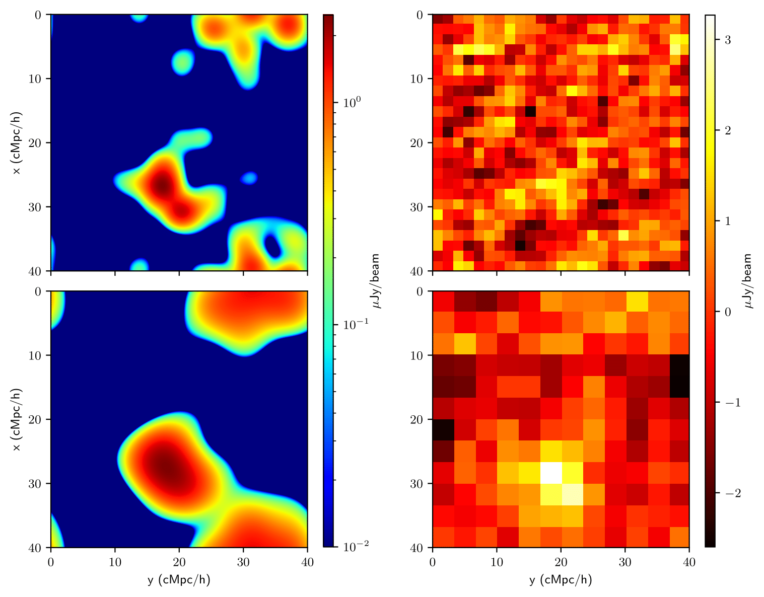
Accounting for angular resolution and thermal noise, in Fig. 9 we show mock radio maps at \(z=4.94\) in CDM for two different angular resolutions, \(\theta_{A} = 1^{\prime}\) and \(\theta_{A} = 2^{\prime}\). Notably, a prominent peak (SNR\(=3.25\)) can be observed in the lower half for \(\theta_{A} = 2^{\prime}\), corresponding to fluxes per beam around \(2 \mu\)Jy. However, enhancing the angular resolution comes at a trade-off of increased thermal noise. This effect is depicted in the top panel of Fig. 9. Here, when adopting \(\theta_{A} = 1^{\prime}\), the peak becomes more challenging to distinguish (SNR=\(1.81\)).

Fig. 9: Mock radio maps for CDM with a frequency channel of width \(\Delta \nu = 272\) kHz and synthesized beam FWHM \(\theta_{A} = 1^{\prime}\) (top row) and \(\theta_{A} = 2^{\prime}\) (bottom row). Left column: Specific intensity field \(I_{\nu}(\hat{\mathbf{r}})\) for \(N_{\text{pix}} = 1024\) corresponding to our simulation resolution. Right column: Specific intensity field overlaid with instrumental noise for \(N_{\text{pix}} = 12\) and \(N_{\text{pix}} = 25\), respectively. We construct the noise map following a four-step procedure.

HIGlow Interpolation

The imaging prospects for cFDM cosmologies are similar to CDM, see peak flux and SNR values in Table 4. At our fiducial redshift of \(z=4.94\), we find a trend of decreasing peak flux \(I_{\mathrm{max}}\) for lower values of the axion mass \(m\). We could not verify this trend at all redshifts and thus do not believe that it is of physical origin. However, as a proof of concept, we take advantage of this trend and demonstrate the ability of HIGlow to interpolate the latent space of axion masses.

As mentioned in Hassan et al. (2022), assuming that HIGlow correctly captures the conditional distribution, it can be used to generate new samples for conditional parameters on which the model has not explicitly been trained. To this end, we generate \(1000\) HIGlow samples for a synthetic cosmology with \(m=3\times 10^{-22}\) eV and quote the maximum peak flux \(I_{\text{max}}\) among all samples in Table 4. We find that the values are in between the \(m=7\times 10^{-22}\) eV and \(m=10^{-22}\) eV values inferred from the full-box approach, indicating the success of HIGlow to interpolate its conditional latent space after training.

Conclusions

21 cm intensity experiments with future radio telescopes like the SKA offer a promising source of new astrophysical and cosmological information about the post-reionization era. As such, we can expect competitive constraints on the DM particle mass \(m\) and non-cold DM fraction, see e.g. Giri & Schneider (2022). In this work, we model the distribution of neutral hydrogen (HI) using high-resolution hydrodynamical \(N\)-body simulations in CDM and three instances of cFDM cosmologies with axion masses \(m=10^{-22}, 7\times 10^{-22}, 2\times 10^{-21}\) eV, adopting the TNG galaxy formation module. Our focus is on the redshift range \(z=3.42-4.94\). We demonstrate the ability of the emerging ML technique of normalizing flows to learn the relevant features in the HI distribution and illustrate the detectability of the brightest HI peaks using SKA1-Low. We summarize our main conclusions as follows:

1. We observe a trend of decreasing HI abundance \(\Omega_{\text{HI}}\) for smaller axion mass \(m\). Comparing to a range of recent measurements, we show that both CDM and the less extreme cFDM models \(m\sim 10^{-21}\) eV are in good agreement therewith. However, the statistical and systematic errors on the measurements are too large to put competitive constraints on FDM using \(\Omega_{\text{HI}}\) directly.
2. The HI bias \(b_{\text{HI}}^2(k) = P_{\text{HI}}(k)/P_{\text{tot}}(k)\) as inferred from the ratio of the HI and total matter power spectra increases with decreasing axion mass, as previously establish. We identify that it is the higher halo bias in cFDM cosmologies (Dunstan et al. 2011) that leads to increased HI clustering. This is also reflected in the amplitude of the 21 cm power spectrum which is up to \(300\)% higher for the \(m=10^{-22}\) eV model than for CDM at \(z=4.94\), similar to (Carucci et al. 2015). We find that SKA1-Low will be able to discriminate among the \(m=10^{-22}\) eV model and CDM at the \(2\sigma\) confidence level on all scales \(k<80 \ h/\)Mpc resolved by the simulations.
3. We show that the HI frequency distribution \(f_{\text{HI}}(N_{\text{HI}}, X)\) decreases in cFDM cosmologies compared to CDM. Its weak dependence on redshift in the post-reionization era allows to compare to a range of DLA and sub-DLA observations covering a wide redshift range. They show very good agreement with predictions from CDM and the less extreme cFDM models \(m\sim 10^{-21}\) eV, with tensions appearing for the \(m=10^{-22}\) eV model.
4. DLA cross-sections exhibit a simple power law + low-mass exponential cutoff trend for cFDM models \(m\sim 10^{-21}\) eV that is well known for CDM models (Villaescusa-Navarro et al. 2018). For more extreme models with \(m\sim 10^{-22}\) eV, we show that a double power law parametrization provides a better fit. The high median cross-section at the low-mass end can be traced to the high column density of cosmic filaments (Gao et al. 2015). Using the mean DLA cross-section, we estimate the DLA bias \(b_{\text{DLA}}\) and recover the well-known result of increasing DLA bias with increasing redshift. In addition, we find the redshift-independent trend that the DLA bias increases with decreasing axion mass \(m\), from \(b_{\text{DLA}} = 2.3\) for CDM to \(b_{\text{DLA}} = 3.8\) for the \(m=10^{-22}\) eV model at \(z=4.94\). This trend is in agreement with Point 2 and is again a result of the increased halo bias in cFDM cosmologies.
5. The prospects of imaging the brightest HI peaks with SKA1-Low at the fiducial redshift of \(z=4.94\) are moderate (SNR \(>3\)) for angular resolutions \(\theta_A \approx 2\), with a rapidly declining SNR for lower values of \(\theta_{A}\). Our peak SNR estimates are lower than for the comparable study of (Villaescusa-Navarro et al. 2014) who assumed \(911\) stations for SKA1-Low as opposed to \(512\).
6. We demonstrate the ability of normalizing flows, a generative ML model introduced by Agnelli et al. (2010), to capture intricate structures resulting from non-linear physics. We adapt the HIGlow framework (Hassan et al. 2022) to facilitate the conditional generation of HI maps with varying axion masses. We use two validation metrics, HI mass PDFs and HI power spectra. As a proof of concept, we showcase the ability of HIGlow to interpolate its latent space of axion masses to predict the peak flux value for a synthetic cosmology with \(m=3\times 10^{-22}\) eV.

As we advance into the systematics-dominated era and witness the construction of PB-scale radio telescopes such as SKA, in the quest for DM it is imperative to improve the modeling of HI distributions in various CDM and non-CDM cosmologies. In the post-reionization era that we focus on, it is easier to disentangle DM signatures from astrophysical processes, which are poorly understood during the epoch of reionization and cosmic dawn. Observations during (Castellano et al. 2023) and after reionization (Irsic et al. 2023) are thus complementary and will increase the robustness of DM constraints. However, a more comprehensive analysis of astrophysical processes is needed even in the post reionization era to swiftly explore a wide array of galactic and stellar feedback effects that can be marginalized over. Advances in cosmological simulations realizing thousands of astrophysical models (Villaescusa-Navarro et al. 2021) and seminumerical modeling techniques Giri & Schneider (2022) signify a major stride in the pursuit of this goal.