Halos

The high-\(z\) large-scale structure (LSS) refers to the distribution of matter on the largest scales, spanning billions of light years. The cosmic web is a prominent feature of the large scale structure, consisting of a vast network of interconnected filaments and voids that stretch across the universe. It is composed of dark matter and gas, which provide the scaffolding for the visible matter, such as stars and galaxies, to cluster and grow. The filaments of the cosmic web are the densest regions of matter, where galaxies and clusters of galaxies are found. These filaments are separated by vast, low-density voids, which are essentially empty regions of space. Nodes, or knots, form the smallest building block of the LSS. For more details about the cosmic web see this page. Here we focus on virialised halos which are embedded into nodes. FDM has many imprints on the internal properties of halos, which we show by analysing a suite of \(N\)-body simulations of CDM and multiple FDM models (Dome et al 2022).

Halo Density profiles

Halos are first identified using the virialisation condition which is typically estimated using spherical collapse theory by extrapolating the linear theory solution to beyond shell-crossing. With respect to the mean overdensity of the universe, it is given by (Bryan & Norman 1998)

\[\label{e_bryan} \tag{1} \Delta_{\text{vir}} = \frac{18\pi^2+82x-39x^2}{\Omega_0}-1.\]

Halo density profiles are then approximated by the Einasto profile (Einasto 1965),

\[\ln\left(\frac{\rho_E(r)}{\rho_{-2}}\right) = -\frac{2}{\alpha}\left[\left(\frac{r}{r_{-2}}\right)^{\alpha}-1\right].\]

which has three parameters: \(\alpha\), the characteristic or scale radius \(r_s \equiv r_{-2}\) at which the logarithmic slope has the isothermal value of \(-2\), i.e. \(\mathrm{d} \ln{\rho} / \mathrm{d} \ln r|_{r_{-2}} = -2\), and the density at the scale radius \(\rho_{-2}\).

A useful quantity to keep in mind is the concentration of halos, defined as

\[c = \frac{R_{200}}{r_{-2}},\]

i.e. the ratio of \(R_{200}\) to that of the scale radius \(r_{-2}\). As discussed by NFW (Navarro et al 1996)for the case of CDM, \(c\) and \(M_{200}\) do not take on arbitrary values, but correlate in a way that reflects the mass-dependence of halo formation times (Bullock et al 2001). Earlier assembly corresponds to higher characteristic densities, reflecting the larger background density at that epoch. The \(c-M_{200}\) relation is shown below.

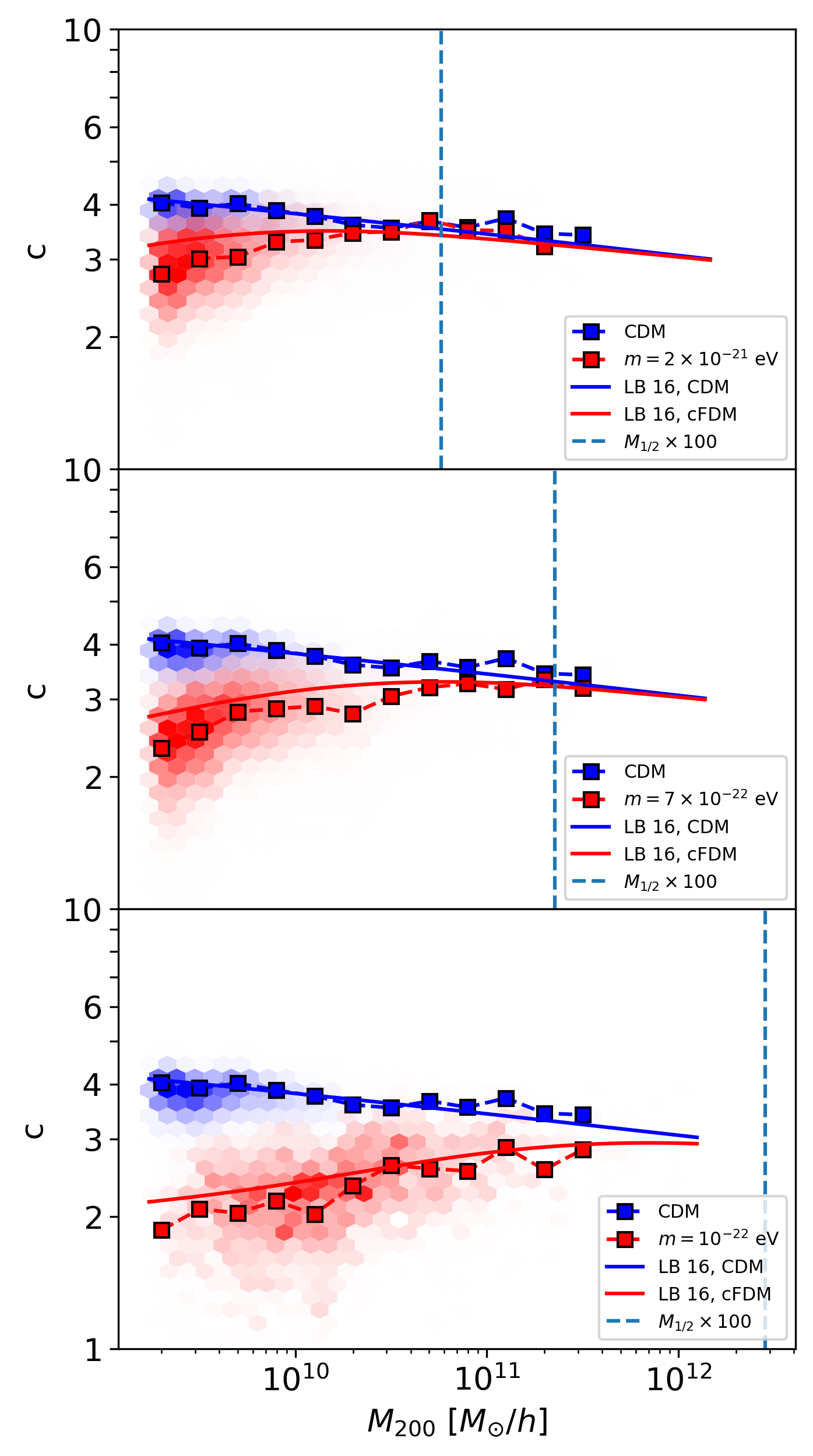
Fig. 1: Concentration-mass relation \(c(M,z)\) in different cosmologies, for \(N\)-body, \(1024^3\) resolution, \(L_{\text{box}} = 40\) cMpc\(/h\) runs at redshift \(z=4.38\). We compare the CDM halos (blue) with cFDM halos for particle mass \(m=2\times 10^{-21}\) eV (top), \(m=7\times 10^{-22}\) eV (middle) and \(m=10^{-22}\) eV (bottom). Square markers indicate median concentrations obtained from Einasto best-fits while the color of each hexbin is proportional to the number of halos whose Einasto concentration falls therein. “LB 16, CDM” and “LB 16, cFDM” show an analytical model prediction from Ludlow et al 2016 for model parameters \(f=0.02\) and \(C=650\).

Ludlow 2014 showed that the concentration of a CDM halo can be inferred from the critical density of the Universe at a characteristic time along its mass accretion history. The insight was used to construct an analytic model for the mass-concentration-redshift relation \(c(M,z)\) for CDM halos, reproducing the inferred relation from many CDM simulations. In Ludlow et al 2016, the generalisation of the model has been introduced and applied to WDM, relying on the full “collapsed mass history” of a halo instead of its main progenitor. As such, the model is based on extended Press-Schechter theory, allowing to assess the dependence of halo concentrations on cosmological parameters and on the shape of the linear matter power spectrum alike. It is this model whose validity for cFDM and high redshifts we would like to comment on.

Fig. 1 shows parts of the \(c(M,z)\) relation as inferred from the \(N\)-body, \(1024^3\) resolution, \(L_{\text{box}} = 40\) cMpc\(/h\) runs at redshift \(z=4.38\). Square markers indicate concentrations as obtained from Einasto best-fits in the respective mass bin, while the color of each hexbin is proportional to the number of halos whose concentration falls therein. The solid blue curve labelled “LB 16, CDM” is a broken power-law fitting formula for \(c(M,z)\) in the Planck cosmology from Ludlow et al 2016 (Eq. C1). At fixed redshift \(z\), the concentrations of CDM halos decrease monotonically with increasing halo mass, reflecting the lower background density at the epoch of their formation. At fixed mass, concentrations \(c\) decrease monotonically with increasing redshift (not shown), indicative of the redshift evolution of the reference density, also called the pseudo-evolution of mass (Diemer et al 2013).

For cFDM, the concentration-mass relation is non-monotonic. In solid red labelled “LB 16, cFDM”, we add the model prediction from Ludlow et al 2016. To maintain consistency, as input to the model we use linear FDM matter power spectra obtained with AxionCamb rather than the Viel et al 2005 parametrisation suitable for WDM. The model parameter \(f\) that is used to define the halo collapse redshift is set to \(f = 0.02\) while the proportionality factor \(C\) relating mean inner halo densities to the critical density of the Universe at the collapse redshift is set to \(C = 650\). We find that their model slightly overpredicts the cFDM concentrations at the small-mass end, while performing better for higher masses. At given \(z\), concentrations peak at around two orders of magnitude above the half-mode mass scale \(M_{1/2}\), with concentrations declining above and below this peak mass scale \(M_{\text{peak}} \sim 100 \times M_{1/2}\). This is a known result which has also been described by e.g. Bose et al 2015. However, both the latter work and that of Ludlow et al 2016 focus on WDM simulations at low redshifts of \(z\leq 3\) and equivalent cFDM particle masses of \(3.3\times 10^{-21}\) eV and \(4.5\times 10^{-22}\) eV. We extend the result to cFDM of lower particle mass of \(m = 10^{-22}\) eV and to redshifts in the range \(3.4 \leq z \leq 6.3\), beyond which our halo catalogues become too sparse and noisy to make statistically robust conclusions. We concede that for the \(m = 1 \times 10^{-22}\) eV run (lower panel), our lack of high-mass halos makes the extrapolation towards \(M_{\text{peak}}\) only tentative.

As in WDM, the non-monotonicity of \(c(M,z)\) is due to the suppression of gravitational collapse below the half-mode scale, breaking the scale-invariance of the assembly process. It imprints a preferred scale on the mass accretion histories. While Ludlow et al 2016 apply their model of the \(c(M,z)\) relation to WDM, here we show that it also fares well for cFDM simulations with initial conditions based on AxionCamb, reproducing the non-monotonicity and even the constancy of \(M_{\text{peak}}\) with cosmic time.

Geometric Halo Alignments

The reason why intrinsic alignments have gained considerable attention in recent years is twofold. First, the next generation of galaxy weak lensing surveys such as the Euclid mission will suffer from highly biased cosmological inferences without a proper alignment modelling informed by simulations and seminumerical methods. At the same time, intrinsic alignments of galaxies provide complementary cosmological information on their own, assuming they can be disentangled from the lensing signal by means of either galaxy color (Yao et al 2020) or polarisation data (Brown et al 2011).

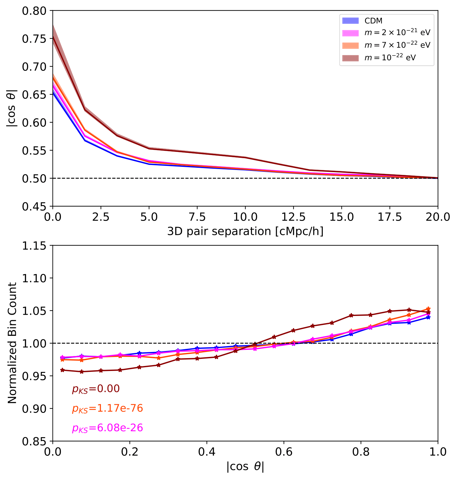
Fig. 2: High-\(z\) shape-position alignment statistics in different cosmologies, for \(N\)-body, \(1024^3\) resolution, \(L_{\text{box}} = 40\) cMpc\(/h\) runs, at redshift \(z=4.38\). We compare CDM halos (blue) to cFDM halos with particle mass \(m=2\times 10^{-21}\) eV (magenta), \(m=7\times 10^{-22}\) eV (dark-red) and \(m=10^{-22}\) eV (orange-red). The results are for intermediate-mass halos in the range \(10^{10}-10^{11} M_{\odot}/h\). Top: Shape-position alignments vs. 3D pair separation, out to \(L_{\text{box}}/2=20\) cMpc\(/h\) to avoid geometric bias induced by the simulation box. Shaded regions enclose the \(25\)th-\(75\)th percentiles. Bottom: PDF of shape-position alignments, with results of the Kolmogorov-Smirnov test of independence between the CDM and cFDM samples.

In Fig. 2, we present shape-position alignment statistics for CDM as compared to cFDM halos at redshift \(z=4.38\), restricted to mass bin \(10^{10}-10^{11} \ M_{\odot}/h\). We find that for large pair separations, the median value for \(|\cos \theta|\) asymptotically approaches \(0.5\), a value consistent with a uniform random shape orientation and halo clustering. For small pair separations, intermediate-mass CDM halos conspire to a median \(|\cos \theta|\) value of around \(0.653^{+0.006}_{-0.002}\), which is in very close agreement with the value Pandya et al 2019 found for real-space 3D mock light cones that they generated for the CANDELS survey at lower redshifts of \(z=1.0-2.5\). What we can also confirm (not shown) is that the shape-shape alignment strength barely reaches values of \(|\cos \theta|\sim 0.6\) for smallest-separation halo pairs, which is systematically lower than the shape-position alignment magnitude.

For cFDM cosmologies, Fig. 2 clearly demonstrates how the geometric alignment is gradually enhanced as the cFDM particle mass \(m\) is decreased. For our most extreme cFDM model with \(m=10^{-22}\) eV, the median \(|\cos \theta|\) curve climbs up to \(0.753^{+0.021}_{-0.010}\), the wider-spread percentiles effected by the smaller number of halos compared to CDM. The enhancement is due to the lack of small-scale structure such as smaller-mass halos that would regularise the tidal fields generated by quasi-linear cosmic filaments and to a lesser extent 2D cosmic sheets. Shape-position alignments are significantly different from the uniform random result even out to 3D pair separations of \(10\) cMpc/\(h\), where \(|\cos \theta| \sim 0.54\). Upon inspection of the \(|\cos \theta|\) distribution after marginalising over 3D pair separations, we find that the Kolmogorov-Smirnov \(p\)-value, \(p_{\text{KS}}\), for rejecting the hypothesis that the cFDM and CDM signals are drawn from the same distribution is very low. In other words, the hypothesis can be ruled out with very high significance. As expected, \(p_{\text{KS}}\) increases with \(m\).

Intrinsic Alignments

While the linear alignment model (LAM) introduced in Hirata et al 2004 and Catelan et al 2001 is traditionally applied to elliptical galaxies, the condition of a virialised, velocity dispersion-stabilised system is also satisfied by halos. To keep our focus on the properties of the cosmic web and to harness greater statistical power, we investigate intrinsic alignment correlations of halos within the LAM. In this model, the halo is assumed to be spherically symmetric in isolation, in a steady-state Jeans equilibrium, perturbed by the presence of a cosmic tidal field. Taylor-expanding the anisotropic large-scale gravitational potential \(\Phi(\mathbf{r})\) to second order around the centre of mass of the halo and assuming that the intrinsic ellipticity \(\epsilon\) can be modelled by a random variable with zero mean and some amount of dispersion, one arrives at

\[\epsilon = \epsilon_{+} + i\epsilon_{\times} = -D(T_{+} + iT_{\times}),\]

i.e. a linear relationship between the local tidal field components \(T_{+}\) and \(T_{\times}\) and the complex ellipticity in projection along the Cartesian \(z\)-axis, \(\epsilon\).

To obtain \(D\) for our simulation samples, we first compute the discrete version of the ellipticity for each halo, see Dome et al 2022. Next, we calculate the local gravitational tidal field

\[\frac{\Phi_{,ij}}{c^2}(\mathbf{x}) = \frac{\partial^2\Phi(\mathbf{x})}{c^2\partial x_i\partial x_j}\]

at the centre of mass of each halo. This can be achieved by first determining the three-dimensional overdensity field \(\delta(\mathbf{x})\) for the full simulation volume using a CIC interpolation. We can then use a discrete Fourier transform to solve Poisson’s equation and obtain the Hessian of the potential algebraically in Fourier space via

\[\frac{\Phi_{,ij}}{c^2}(\mathbf{x}) = \frac{3\Omega_m}{2\chi_H^2a}\mathcal{F}^{-1}\left[ \frac{k_ik_j}{|\mathbf{k}|^2} \exp\left(-\frac{1}{2}|\mathbf{k}|^2\lambda^2\right)\mathcal{F}[\delta(\mathbf{x})]\right],\]

where \(\mathbf{k}\) is the comoving wave vector, \(\chi_H = \frac{c}{H_0}\) is the Hubble-distance and \(a\) the cosmic scale factor. There is a non-removable uncertainty on the scale the effective tidal field relevant for LAM should be evaluated on. Here, we consider a Gaussian smoothing scale of \(\lambda =\) 1 cMpc/\(h\). This scale corresponds to halos of mass \(M = 4\pi/3 \Omega_m \rho_{\mathrm{crit}} \lambda^3 \sim 10^{11} \ M_{\odot}/h\). Finally, to obtain the tidal shear at the halo positions, we perform an inverse CIC interpolation, effectively increasing the smoothing scale \(\lambda\) by about one grid cell.

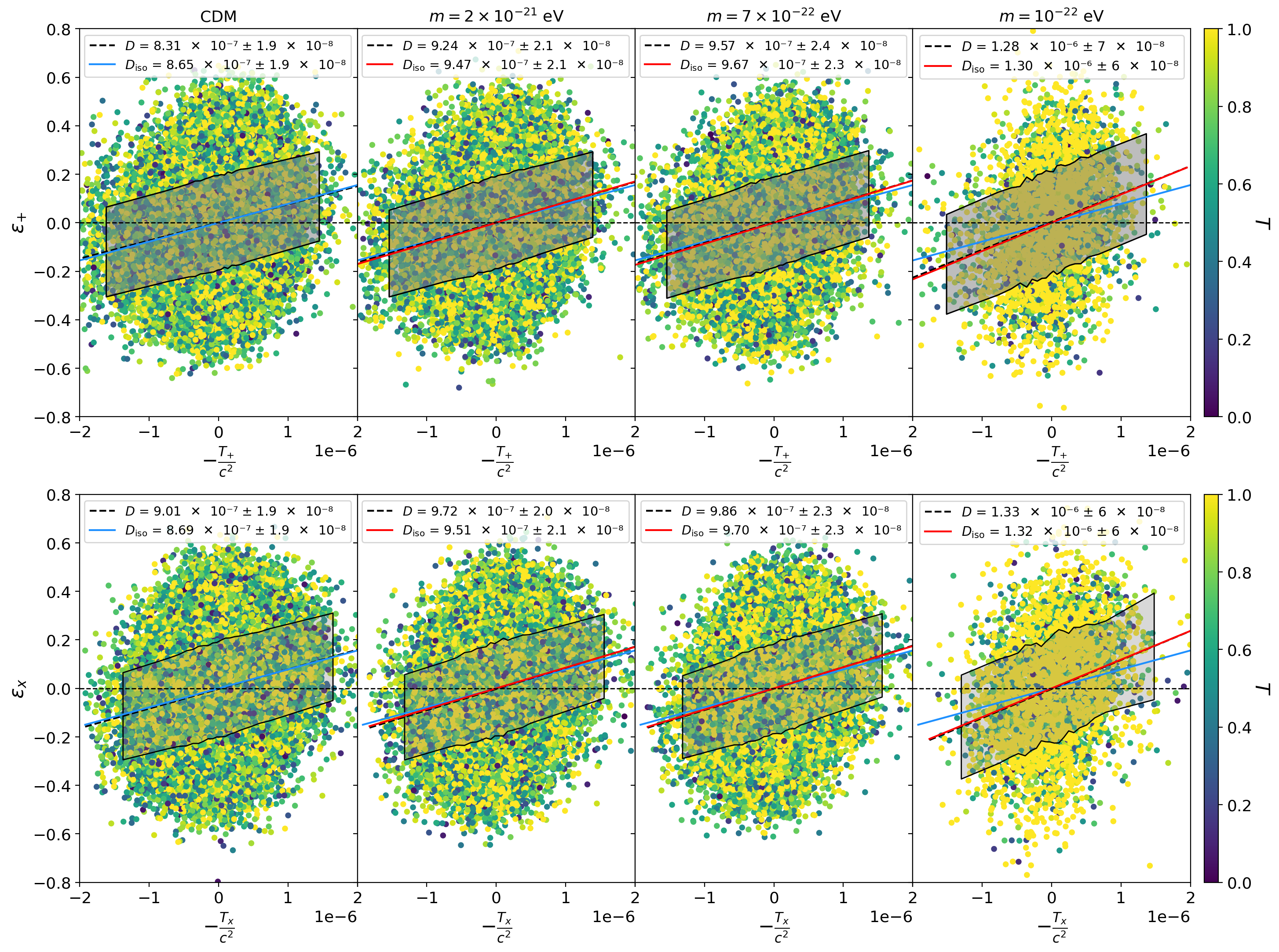
Fig. 3: Intrinsic alignment strengths in different cosmologies. We show the correlation of the two components of the halo ellipticity \(\epsilon_{+}\), \(\epsilon_{\times}\) with the respective tidal field components \(T_{+}\), \(T_{\times}\), for \(N\)-body, \(1024^3\) resolution, \(L_{\text{box}} = 40\) cMpc\(/h\) runs at redshift \(z=4.38\). Each dot represents one halo colour-coded by its triaxiality \(T\). The blue dashed lines correspond to a linear fit to the binned data points, the shaded bands displaying the standard error on the mean (SEM) in each bin. The blue (CDM) and red solid lines (cFDM) depict the fits to the anisotropy-corrected data. All values are in units of \(c^2(\mathrm{cMpc}/h)^2\).

In Fig. 3, we present some selected best-fit results for the alignment parameter \(D\). We quote isotropised values \(D_{\text{iso}}\) rather than the raw \(D\) values. As we decrease the cFDM particle mass \(m\), one noticeable change in Fig. 3 comes from the higher average in the triaxiality \(T\) of halos. By the same token, the distributions of both the real and the imaginary part of the ellipticity \(\epsilon_{\times}\) exhibit more outliers / heavier tails at larger absolute values than for CDM. This is expected, since prolate halos tend to look - on average - prolate in projection as well. This circumstance together with the distribution of local tidal field values \(T_{+}\), \(T_{\times}\), conspire to a strong dependence of the alignment strength on the cFDM particle mass \(m\). The smaller \(m\) and thus the smaller the half-mode scale \(k_{1/2}\), the more \(D_{\text{iso}}\) grows. The fractional difference in \(D_{\text{iso}}\) between the most extreme cFDM model with \(m=10^{-22}\) eV and CDM is as high as \(0.45 \pm 0.19\) at \(z=10.9\). At \(z=4.38\), the fractional difference reads \(0.51\pm 0.08\), which is different from zero at a level of about \(6.4 \sigma\).