Cosmic Web

On scales of \(1-100\) Mpc the matter distribution of the Universe forms a weblike pattern of voids separated by walls, filaments and nodes - the cosmic web (Bond et al. 1996). The most prominent features of the cosmic web are filaments, and beyond the well-known Pisces-Perseus chain (Giovanelli & Haynes 1985) in the local Universe, entire filament inventories have been catalogued (Tempel et al. 2014). The largest filaments act as highways of the Universe, channelling dark matter, gas and galaxies into the higher density node regions. The nodes contain the highest density of galaxy clusters and superclusters such as the Great Attractor (Lynden-Bell et al. 1988), the Shapley concentration (Ragone et al. 2006) or the Vela supercluster (Kraan-Korteweg et al. 2017).

The 2D components of the cosmic web, sheet-like membranes, are more difficult to detect in the spatial mass distribution traced by galaxies due to their lower surface density. The spatial structure outlined by galaxy clusters, however, does feature flattened supercluster configurations coined great walls, the most outstanding of which are the CfA Great Wall (Geller & Huchra 1989), the Sloan Great Wall (Gott et al. 2005), the BOSS Great Wall (Lietzen et al. 2016) and the supergalactic plane (Lahav et al. 2000). Finally, large void regions are prominent features in redshift surveys as they are practically devoid of any galaxy. Recent studies (Leclercq et al. 2015) provide increasingly refined maps and catalogues of the void population in the local Universe. Out of all known voids, the Local Void with a diameter of 30 Mpc is closest to the Milky Way.

At high redshift, the Universe evolves mostly linearly, i.e. linear relativistic (or Newtonian) perturbation theory (PT) still provides an accurate description of gravitational collapse in an expanding Universe. When applying linear PT to a Gaussian field, which provides an accurate description of primordial density fluctuations in the early Universe, one finds that different wavelength modes do not couple; they evolve independently. The cosmic web is still in the linear or quasi-linear phase of collapse. Since FDM on large scales (including halo scales) is most manifest in an effective small-scale cutoff of the primordial density fluctuations, i.e. affecting small-scale modes, FDM imprints on the cosmic web at high-\(z\) are especially pronounced. These imprints are only observable via tracer fields, but in simulations we can predict the configuration and abundance of each morphological component in CDM and FDM.

On this page we show results for the cosmic web dissection of numerical CDM and cFDM simulations into the four morphological components. This is work based on Dome et al. (2022). For more details about the internal properties of halos embedded in the densest component (i.e. nodes) in CDM and FDM see this page.

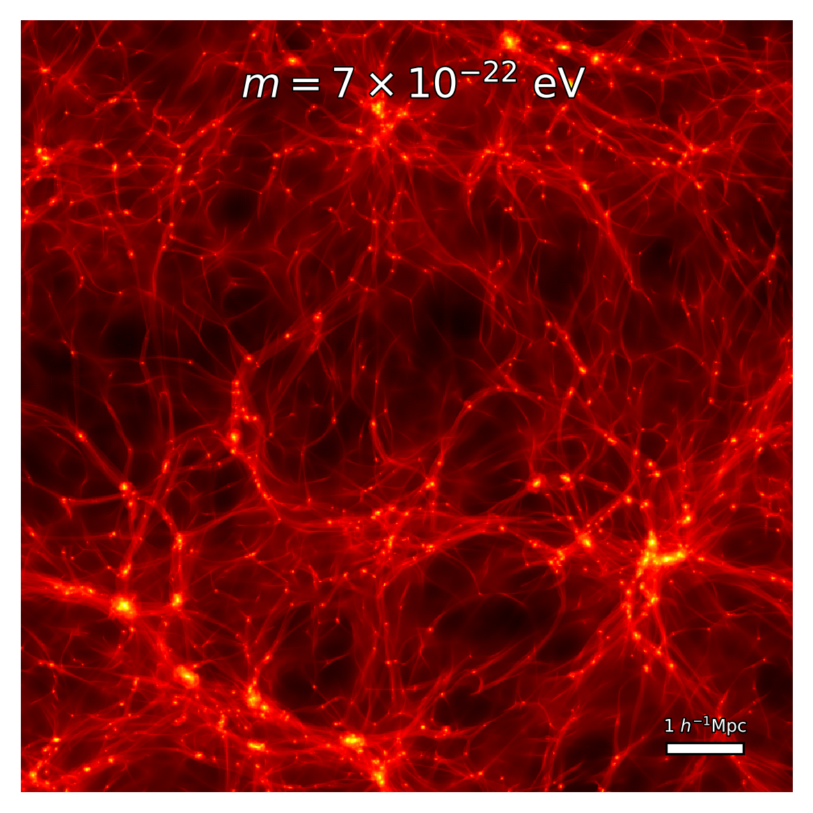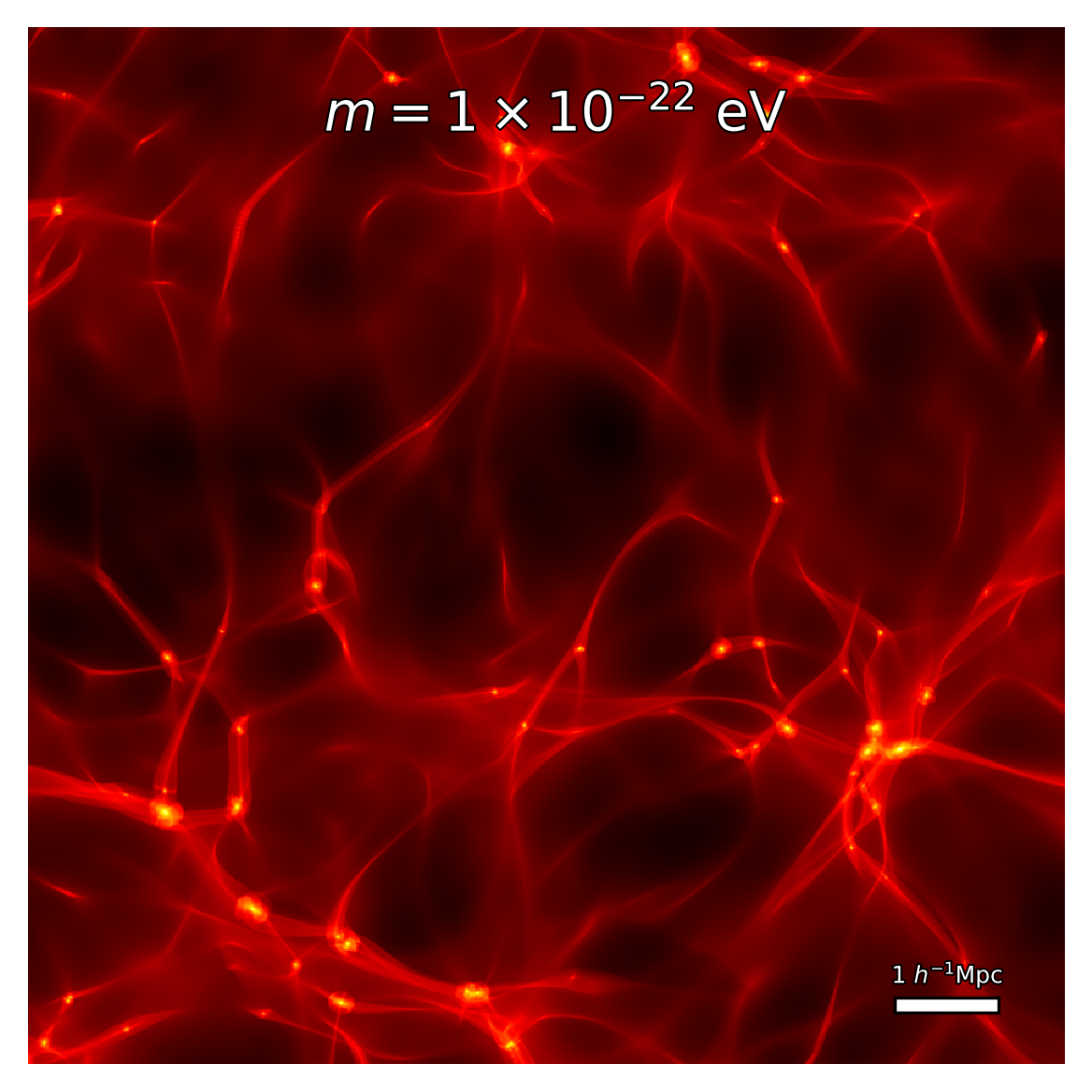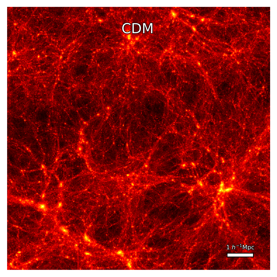
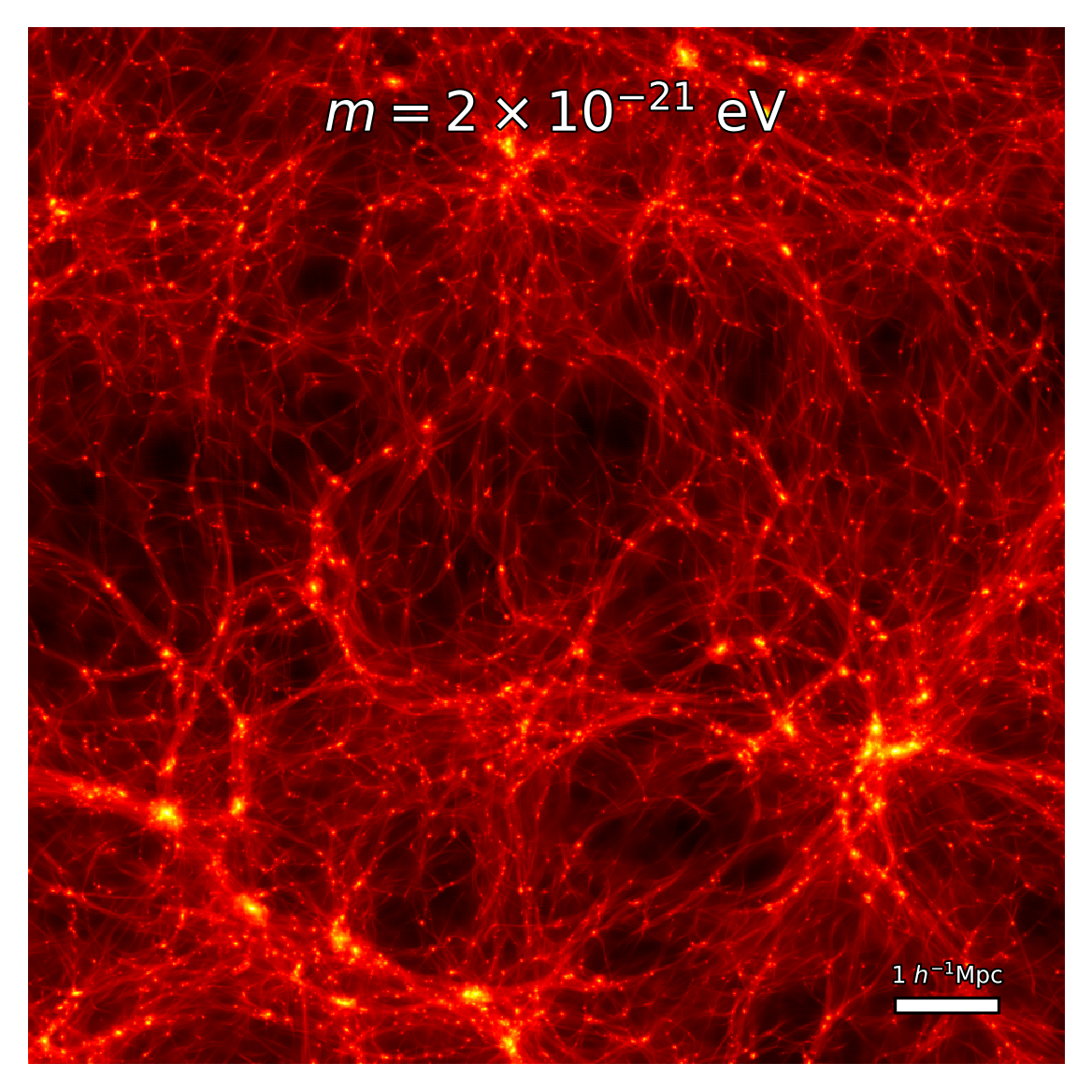
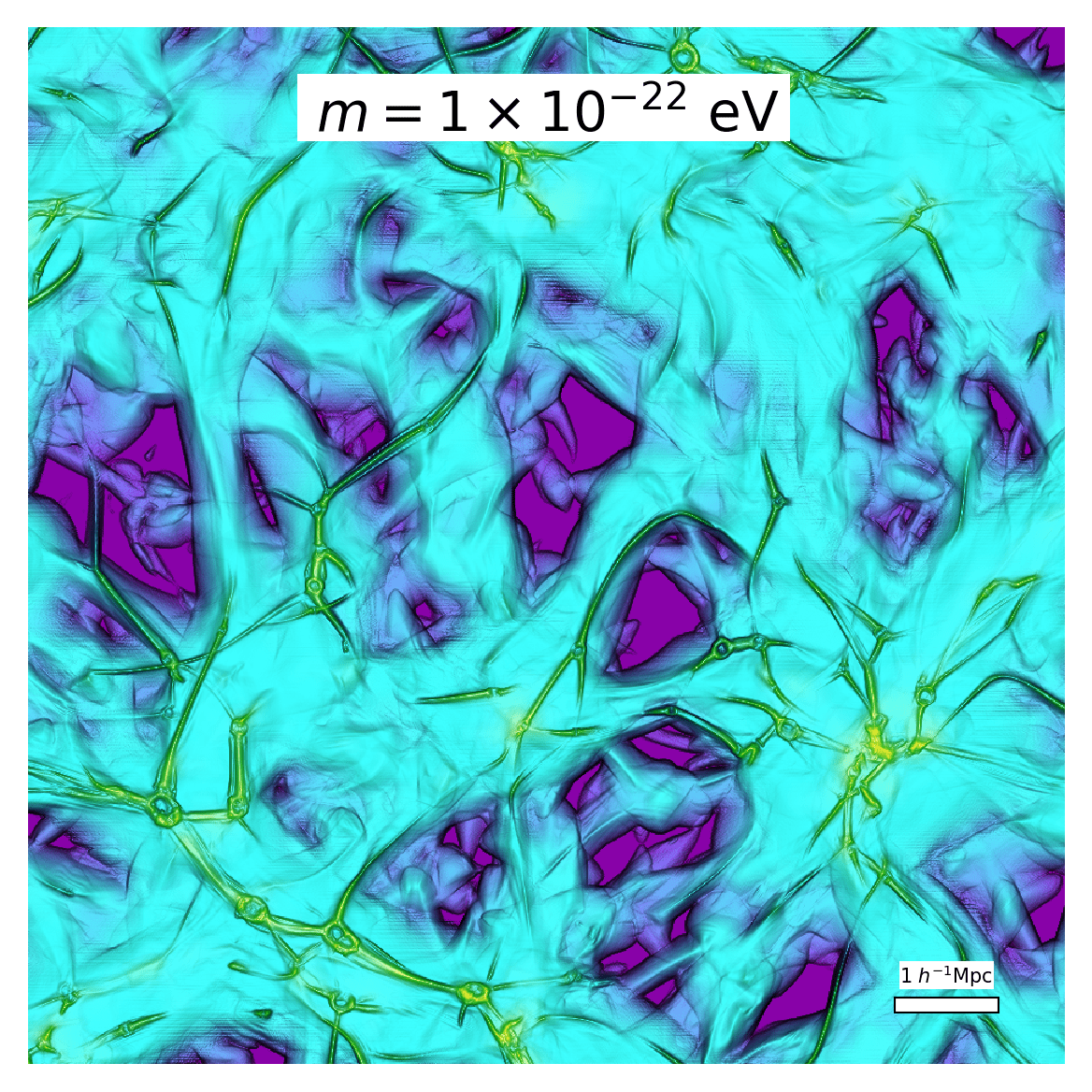
Fig. 1: Comoving DM density field in a \(9 \times 9 \times 9 \ (h^{-1}\text{Mpc})^3\) volume of the \(N\)-body CDM (top left) and cFDM (\(m=2\times 10^{-21}\) eV run: top right, \(m=7\times 10^{-22}\) eV run: bottom left and \(m=10^{-22}\) eV run: bottom right) runs with \(1024^3\) resolution and \(L_{\text{box}} = 10\ h^{-1}\)Mpc at \(z=3.9\), shown in logarithmic projection.

Density field projections in various cosmologies are shown in Fig. 1, for the exemplary redshift of \(z = 3.9\). On scales much larger than the local de-Broglie wavelength \(\lambda_{\text{dB}}\), CDM can be thought of as a limiting case of FDM in the following sense: The FDM potential field converges to the classical answer as \(\mathcal{O}(\hbar/m)^2\), thus any superfluid dynamics recovers the classical collisionless limit as \(\hbar/m \rightarrow 0\), even in the case of multi-stream flows. However, the density field fails to converge due to order unity fluctuations driven by interference and the uncertainty principle (Mocz_2018). Mathematically, there is no exact correspondence between the Schrödinger-Poisson and the Vlasov-Poisson equation since the former describes a fluid while the latter collisionless particles. FDM remains a fluid even for \(\hbar/m \rightarrow 0\). This quasi-correspondence between FDM and CDM in the large-\(m\) limit, or rather, the $exact$ correspondence between cFDM and CDM, is visible in the density field projections of Fig. 1. They illustrate how small-scale power is suppressed as the axion mass is reduced from infinity (CDM, top left) all the way down to \(m=10^{-22} \ \text{eV}\) (bottom right).

NEXUS Segmentation

Cosmic web detection algorithms can be categorised into graph- and percolation-based techniques (Naidoo et al. 2022), stochastic methods (Stoica et al. 2010), topological methods (Aragón-Calvo et al. 2010) and Hessian-based approaches, see Libeskind et al. (2017) for a comparison. Our focus in the following is on Hessian-based approaches which exploit morphological information in the gradient (or Hessian) of the density, tidal or velocity shear fields. Most of the Hessian-based formalisms are defined on one particular smoothing scale for the field involved (Bond et al. 2010), but explicit multiscale versions have also been developed, including (Aragón-Calvo & Jones 2007).

In this work we use NEXUS+. NEXUS+ is likewise a morphological multiscale approach based on the density field Hessian. By log-smoothing the density field over a range of spatial filter sizes \(R_n \in (R_0, ..., R_N)\) and maximising over the signatures in this so-called scale-space, it detects at which scales and locations the various morphological signatures are most prominent. The six steps of the algorithm along with our implementation choices are as follows.

1. Applying a log-Gaussian filter of width \(R_n\) to the input field. If the input field is continuous and denoted by \(f(\vec{x})\), smoothing the log-field \(g = \log_{10} f\) amounts to a simple multiplication with the Gaussian exponential in Fourier space:

   \[g_{R_n}(\vec{x}) = \int_{\mathbb{R}^3} \frac{d^3\vec{k}}{(2\pi)^3}e^{-\vec{k}^2\frac{R_n^2}{2}}\hat{g}(\vec{k})e^{i\vec{k}\vec{x}}.\]

   This yields the NEXUS+ smoothed field \(f_{R_n}(\vec{x}) = C_{R_n}10^{g_{R_n}(\vec{x})}\) by exponentiation, where \(C_{R_n}\) assures the mean of the input field is the same before and after filtering.

2. Computing Hessian eigenvalues. The Fourier transform of the Hessian \(H_{ij,R_n}(\vec{x})=R_n^2\frac{\partial^2 f_{R_n}(\vec{x})}{\partial x_i \partial x_j}\) reads

   \[H_{ij,R_n}(\vec{k})=-k_ik_jR_n^2\hat{f}_{R_n}(\vec{k}).\]

3. Assigning to each point a cluster, filament and wall signature. The three eigenvalues \(\lambda_1 \leq \lambda_2 \leq \lambda_3\) of the Hessian \(H_{ij,R_n}(\vec{x})\) can be combined into a shape strength as

   \[\mathcal{I}_{R_n} = \begin{cases} \ \big|\frac{\lambda_3}{\lambda_1} \big| & \text{node} \\ \ \big|\frac{\lambda_2}{\lambda_1} \big| \Theta\left(1-\big|\frac{\lambda_3}{\lambda_1} \big|\right) & \text{filament}\\ \ \Theta\left(1-\big|\frac{\lambda_2}{\lambda_1} \big|\right) \Theta\left(1-\big|\frac{\lambda_3}{\lambda_1} \big|\right) & \text{wall}, \end{cases}\]

   where we use the notation \(\Theta(x) = x\theta(x)\) for clarity, with \(\theta(x)\) the Heaviside step function \(\theta(x) = 1\) if \(x \geq 0\), \(0\) otherwise. We thus obtain the cluster/filament/wall signature as:

   \[\mathcal{S}_{R_n} = \mathcal{I}_{R_n}\times \begin{cases} \ |\lambda_3|\theta(-\lambda_1)\theta(-\lambda_2)\theta(-\lambda_3) & \text{node} \\ \ |\lambda_2|\theta(-\lambda_1)\theta(-\lambda_2) & \text{filament}\\ \ |\lambda_1|\theta(-\lambda_1) & \text{wall}. \end{cases}\]

   We multiply by \(|\lambda_i|\) to distinguish between noise (small \(|\lambda_i|\)) and real signals (large \(|\lambda_i|\)) while the \(\theta(-\lambda_i)\) factors impose the necessary eigenvalue constraints.

4. Computing the environmental signature over a range of smoothing scales. We repeat steps 1-3 over a range of smoothing scales \((R_0, R_1, ..., R_N)\). While NEXUS+ is a multi-scale approach, the hierarchy of smoothing scales is a user input. In view of computational feasibility, we opt for relative \(\sqrt{2}\)-spacings following Cautun et al. (2012), i.e. \(R_n = (\sqrt{2})^nR_0\), where \(R_0\) is the smallest scale at which to expect to find structures. We comment on \(R_0\) and the discretization of \(f(\vec{x})\) below while \(N\) is chosen such that \(R_N\) does not exceed \(4 \ h^{-1}\)Mpc. At higher redshift of \(z>1\), smaller values for \(R_N\) would suffice.

5. Scale-space stacking. The scale-independent map is constructed by taking the maximum signature over all scales

   \[\mathcal{S}(\vec{x}) = \max_{\text{levels } n} \mathcal{S}_{R_n}(\vec{x}),\]

   which characterizes the degree to which each voxel \(\vec{x}\) is part of a cluster, filament or wall.

6. Computing the detection threshold. As the last step, we impose physical criteria to determine the detection threshold corresponding to valid environments. For nodes, the threshold signature \(\mathcal{S}_{c,\mathrm{cut}}\) is found by requiring that at least half of the connected regions are virialised according to this page, Eq. 1. This is in contrast to the original papers Cautun et al. (2012) and Cautun et al. (2014), where the authors use a virialisation overdensity of \(\Delta_{\text{vir}} = 370\). To identify connected regions for each node signature floor \(\mathcal{S}_{c}\), we label them based on a \(1\)-connectivity neighbourhood condition. The value \(1\) refers to the maximum number of orthogonal hops to consider a voxel a neighbour.

   Voxels that do not pass this threshold are assigned a node signature of zero. Voxels that do pass the threshold constitute genuine node structures, and after setting the real-space density values at their location to the mean density of the Universe (rather than zero as in Cautun et al. (2012)), the slightly modified input field \(\tilde{\delta}(\mathbf{x})\) becomes the basis for the calculation of filament signatures \(\mathcal{S}_{f,R_n}(\mathbf{x})\) in step 3. The procedure is similar to the one for nodes, except that for filaments, the threshold signature is determined by calculating the mass \(M_f(\mathcal{S}_f)\) in filaments with a signature value larger or equal to \(\mathcal{S}_f\) and maximizing the mass change with signature:

\[\label{e_fw_det} \tag{1} \mathrm{argmax}_{\mathcal{S}_f} \ \bigg\lvert \frac{\mathrm{d}M_f^2}{\mathrm{d}\log \mathcal{S}_f}\bigg\rvert = \mathcal{S}_{f,\mathrm{cut}}.\]

After identifying filaments and setting the real-space density values at their location to the mean density of the Universe, we identify walls using the same detection threshold, Eq. \(\ref{e_fw_det}\). The remaining voxels are automatically identified as voids, which thus constitute the complement to nodes, filaments and walls.

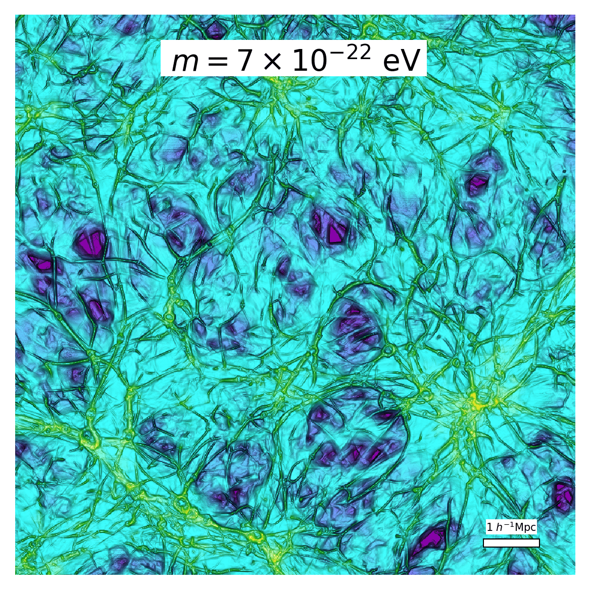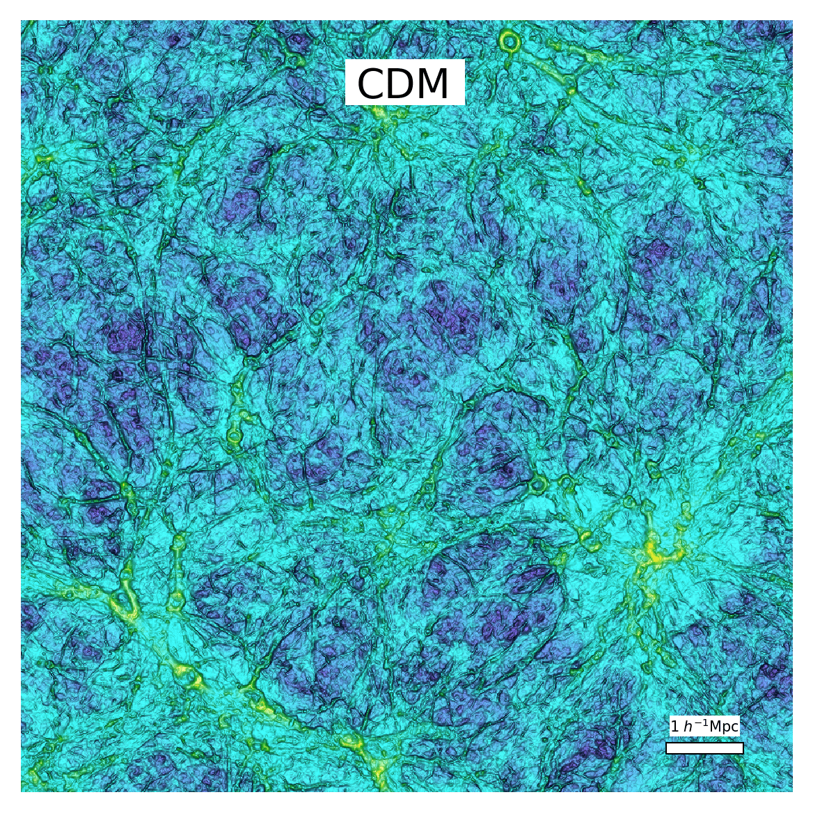
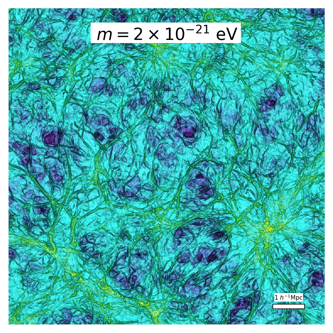
Fig. 2: An illuminated 2D projection of the filamentary NEXUS+ network \(\mathcal{S}_f(\mathbf{x})\) after scale-space stacking and imposition of \(\mathcal{S}_{f,\mathrm{cut}}\) in logarithmic projection at redshift \(z=3.9\) in a \(9 \times 9 \times 9 \ (h^{-1}\text{Mpc})^3\) volume (corresponding to Fig. 1) of the \(N\)-body CDM (top left) and cFDM runs (\(m=2\times 10^{-21}\) eV run: top right, \(m=7\times 10^{-22}\) eV run: bottom left and \(m=10^{-22}\) eV run: bottom right) with \(1024^3\) resolution and \(L_{\text{box}} = 10 \ h^{-1}\)Mpc.

For the above set of parameter choices and definition of signature thresholds, Fig. 2 shows a 2D projection of the filament signature field \(\mathcal{S}_f(\mathbf{x})\) after scale-space stacking and after imposition of the threshold signature \(\mathcal{S}_{f,\mathrm{cut}}\). The intricate filigree of filaments surrounded by vast empty regions is well discernible in Fig. 2, as well as filamentary signatures being zero at the location of cosmic nodes. This is expected since each voxel receives only one labelling: node, filament, wall or void. As the axion mass \(m\) is gradually reduced, the primordial power spectrum cutoff migrates to a larger spatial scale. Concomitant with this migration, we observe a gradual removal of the thinnest filaments. In addition, we find that filaments become visually smoother, which is related to smoother DM accretion onto halos (Khimey et al. 2021).

Cosmic Web Statistics at High Redshift

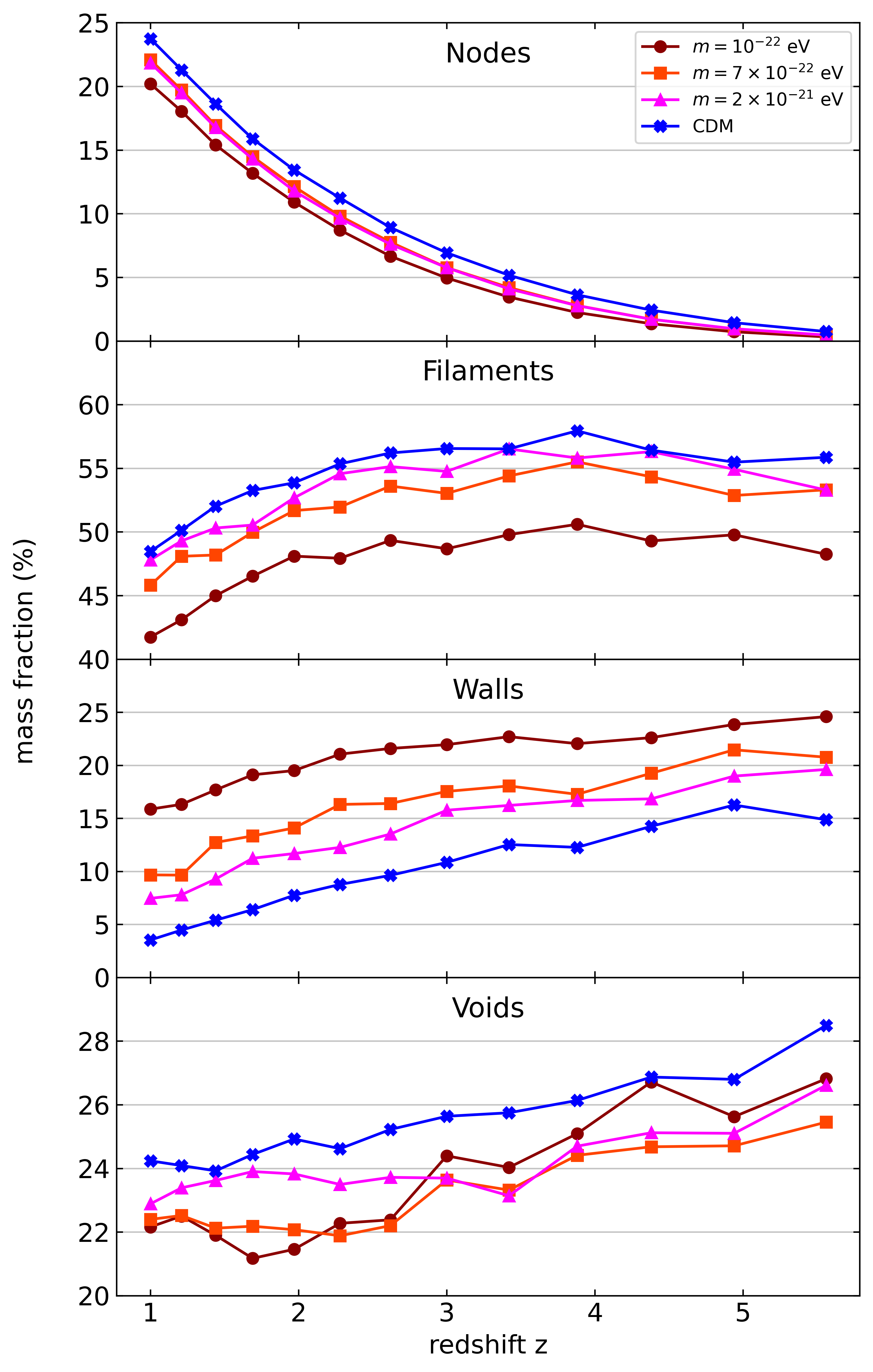
One way of characterising the cosmic web evolution is by tracking mass and volume filling fractions of each of its components. Since each voxel is assigned only one component label, this exercise is trivial and amounts to summing up the mass or volume contained in all component voxels. We show the result in Fig. 3 for CDM vs cFDM. To understand the evolution of the cosmic web environments in CDM, the works of Shandarin & Zeldovich (1989) and van de Weygaert & Bond (2008) provide good guidance: They show how matter flows out of voids towards walls, inside of which it streams towards filaments at the edges of these planar structures, which in turn channel matter towards node regions. In this simple picture which is corroborated by large-scale velocity field studies in Cautun et al. (2014), voids always lose mass while nodes always become more massive, establishing two opposite-trended monotonicity relations in the mass filling fractions of voids and nodes as visible in Fig. 3.

Even though walls experience both inflow and outflow of matter just as filaments, they tend to be described by decreasing mass and volume fractions at both high and low redshift. Two-dimensional sheets (walls) contain \(\sim 10\)% less mass and volume at \(z=1\) than at \(z= 5.6\) in both CDM and cFDM. By contrast, filaments tend to keep their mass filling fractions fairly constant across cosmic time until \(z\sim 3\), below which they start decreasing. Their volume fractions decrease gradually, from around \(\sim 28\)% at \(z= 5.6\) to around \(\sim 13\)% at \(z=1\). This suggests that similar mass fractions get accumulated into fewer, but more massive filaments. With the largest share of mass, cosmic filaments play a critical role in the formation of galaxies, co-determining their spin and spatial distribution, see Malavasi et al. (2020) and Poudel et al. (2017). It stresses the importance of revisiting standard theories which assume that halo environments in which protogalaxies form play the dominant role in shaping the properties of galaxies, see e.g. Wilman et al. (2012) and Behroozi et al. (2010).

How DM is distributed across different components of the cosmic web depends on the DM model at hand and thus the cosmology. Here we find that the lower the axion mass \(m\), the lower the relative share of mass in nodes and filaments and the higher the mass share in walls when compared to CDM. To be precise, the mass filling fraction of filaments exhibits a \(\sim 6-8\)% decrease between CDM and the \(m=10^{-22}\) eV model across most of the redshifts investigated. This is mainly compensated for by a \(\sim 8-12\)% increase in mass filling fractions of walls between CDM and the \(m=10^{-22}\) eV model. The redistribution of DM to higher-dimensional structures, i.e. sheets, is a manifestation of the loss of small-scale power in the primordial and also evolved DM distributions.

Fig. 3: Evolution of the mass (left) and volume (right) filling fractions for the \(N\)-body CDM and cFDM runs with \(1024^3\) resolution and \(L_{\text{box}} = 40\ h^{-1}\)Mpc. Each row represents a different NEXUS+ cosmic web environment. Cosmologies are differentiated by color as shown in the legend.

The DM budget in each cosmic web environment also affects large-scale tidal forces in the Universe, shaping the evolution of halos and galaxies. In the same way that tidal torque theory predicts quadrupolar patterns in the vorticity field around the saddle points of cosmic filaments (Codis et al. 2015), tidal forces give rise to dipolar patterns around cosmic sheets. Consequently, such dipolar features are expected to be more pronounced in cFDM cosmologies than in CDM. Sheet-like morphologies are attributed increased importance in the gas dynamics of FDM as well, since massive gas pancakes are predicted to be the sites of first star formation (Kulkarni et al. 2022). Note, however, that global mass filling fractions are anisotropy-agnostic and by construction gloss over the enhanced matter distribution anisotropies apparent in cFDM cosmologies (Dome et al 2022). Reliable tidal force predictions would necessitate an analysis of anisotropic geometries and are thus beyond the scope.

Overdensity PDFs

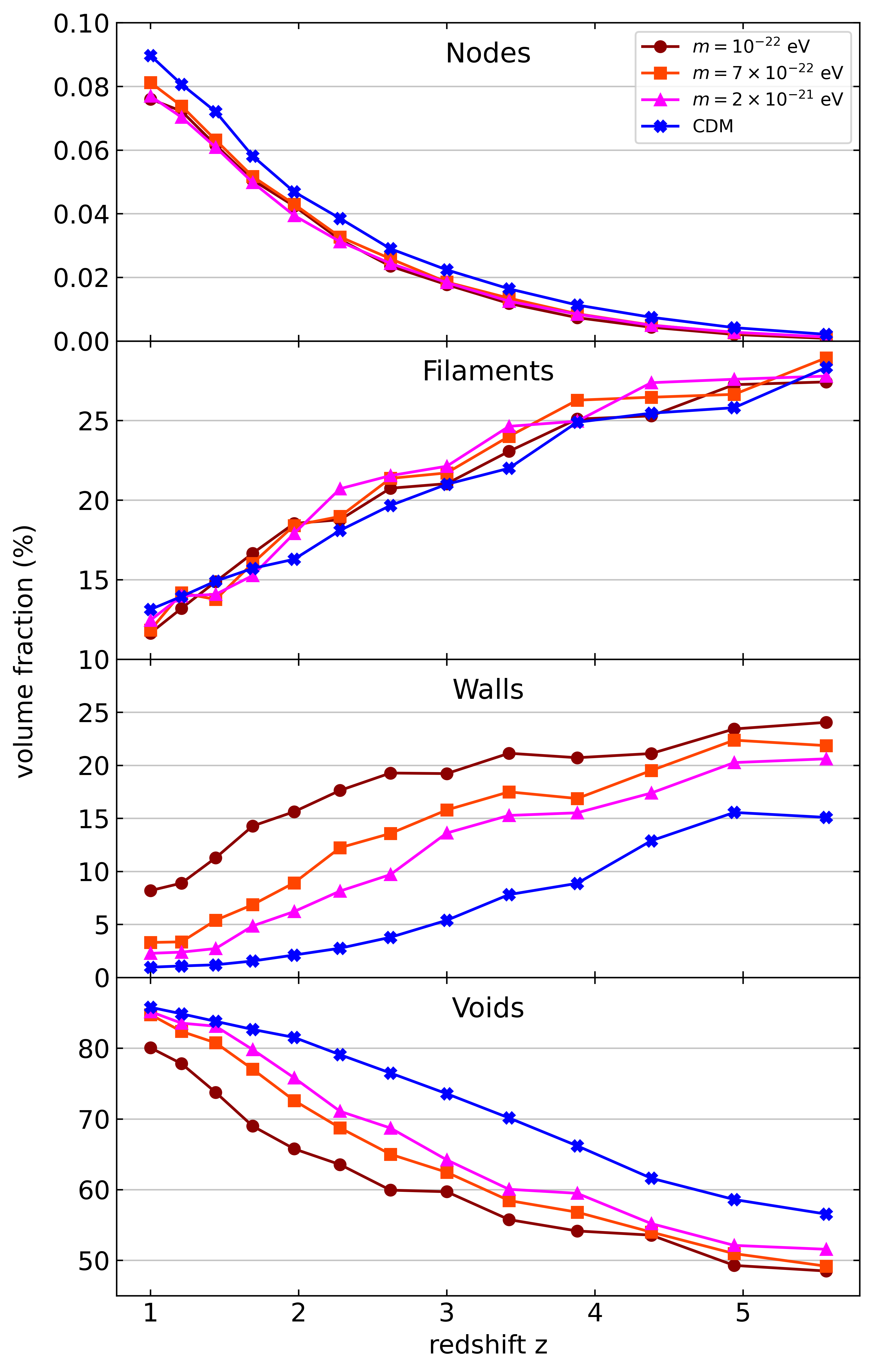
The simplest way of characterising the variation of the matter content across environments is via density distributions. As in the rest of this work, we use the CIC density to obtain the probability density function (PDF) of the log overdensity field \(\log_{10}(1 + \delta)\). In Fig. 4, the PDF is segmented into morphological components.

Fig. 4: Log overdensity PDFs for the \(N\)-body CDM and cFDM runs with \(1024^3\) resolution and \(L_{\text{box}} = 40\ h^{-1}\)Mpc at redshift \(z=3.9\). Cosmologies are differentiated by color as shown in the legend. The first four rows represent different NEXUS+ cosmic web environments while the last row shows the overall log overdensity PDFs. The dashed green curve (fourth row) is the CDM best-fit result using the Miralda-Escudé et al. (2000) fitting formula for the void log overdensity PDF while the dashed cyan curve (bottom row) is the CDM best fit among the family of reversed Weibull distributions, cf. Repp & Szapudi (2018).

Let us again start the discussion with CDM. We find that various cosmic environments are characterised by different values of the log overdensity field. Node regions have by far the highest PDF median at around \(1+\delta \sim 300\). Filaments also predominantly represent overdense environments as can already be predicted within the Zel’dovich formalism (Pogosyan et al. 1998 and has been found by e.g. Aragón-Calvo et al. 2010. Walls and especially voids are more likely to be found in underdense environments. The large widths of the distributions give rise to significant overlaps between the log overdensity PDFs of different components. A simple density threshold (Dolag et al. 2006) is thus only sufficient to identify cosmic nodes but cannot be used to differentiate between the remaining components.

The cFDM models show significantly narrower distributions around the median values than in CDM, except for node environment PDFs which are fairly insensitive to a primordial power spectrum cutoff. Filament environment PDFs, for instance, have their full width at half maximum (FWHM) decrease from \(0.94\) dex for CDM to \(0.50\) dex for \(m=10^{-22}\) eV cFDM. For the overall PDFs (last row in Fig. 4), the corresponding numbers read \(0.84\) dex vs \(0.55\) dex. Intuitively, this can be explained as follows: In the case of filaments, small-scale structure is typically associated with tenuous tendril-like features or substructure at the periphery of more major filaments, which get washed out as the axion mass \(m\) gets reduced. The suppression of the high-overdensity tail results from the delayed formation of large-scale structure and high-mass halos in particular compared to CDM, see e.g. Safarzadeh et al. (2018). This effect is most striking for walls which in cFDM have a higher share of mass, see Fig. 3. With suppression at both ends, the PDF is more narrow. For all environments except nodes, the narrower distribution with a strong mid-range peak illustrates that density minima are more shallow. In the case of voids, this is a well-known result (Yang et al. 2015) that is independent of the adopted cosmic web dissection algorithm.

Cosmic Skewness

In order to gain insight into the asymmetries of the overdensity distribution function, we briefly focus on the third moment of the unconditioned PDF \(P(\delta)\), also known as skewness.

The definition of PDF moments that is most widely adopted in the cosmological literature (Bernardeau et al. 2002) is

\[S_p = \langle \delta^p \rangle / \langle \delta^2 \rangle^{p-1},\]

where

\[\langle \delta^p \rangle = \int_{-1}^{\infty}\mathrm{d}\delta P(\delta)\delta^p,\]

and accordingly \(S_3 = \langle \delta^3 \rangle / \langle \delta^2 \rangle^2\). The overdensity distribution function \(\mathrm{d}N/\mathrm{d}\delta = P(\delta)\) is defined as the normalised number of elements of the density field with a density contrast in [\(\delta, \delta + \mathrm{d}\delta\)], and is thus related to the log PDF via

\[\frac{\mathrm{d}N}{\mathrm{d}(\delta + 1)} = \frac{1}{\ln(10)}\frac{\mathrm{d}N}{(\delta + 1)\mathrm{d}\log_{10}(\delta + 1)}.\]

Physically, \(S_3\) measures the tendency of gravitational clustering to create an asymmetry between underdense and overdense regions. As clustering proceeds, there is an increased probability of having large values of \(\delta\) compared to a Gaussian distribution, leading to an enhancement of the high-density tail of the PDF \(P(\delta)\). As underdense regions expand and most of the volume becomes underdense, the maximum of the PDF shifts to negative values of \(\delta\), and one can show (Bernardeau et al. 2002) that the maximum of the PDF to first order in the square root of the cosmic matter variance \(\sigma = \sqrt{\langle \delta^2 \rangle}\) is reached at

\[\delta_{\mathrm{max}} \sim -\frac{S_3}{2}\sigma^2,\]

providing useful information about the shape of the PDF.

We obtain error estimates on \(S_3\) through jackknife resampling: The full simulation box of side length \(L_{\text{box}} = 40\ h^{-1}\)Mpc is divided into \(4^3\) equal-sized subcubes, each time omitting one of the small cubes while calculating the statistical moments. The jackknife standard variance we adopt is

\[\hat{\mathrm{var}}(\hat{\theta}_{\mathrm{jack}}) = \frac{1}{N}\frac{1}{N-1}\sum_{i=1}^{N}\left(\mathrm{PV}(\mathrm{x}_{(i)})-\overline{\mathrm{PV}}\right)^2.\]

Here, \(\mathrm{x}_{(i)}\) denotes the sample but with the \(i^{\mathrm{th}}\) observation removed. In our case, this translates to a subbox removal. Each pseudo-value \(\mathrm{PV}(\mathrm{x}_{(i)})=n\hat{\theta}-(n-1)\hat{\theta}_{(i)}\), can be viewed as an estimate of \(\theta = S_3\), and it is their variance that determines the jackknife standard error.

We focus on the overall skewness \(S_3\) as is common, without conditioning on cosmic environment. The evolution of both the CDM and cFDM model Universes starts off from a Gaussian random field that is symmetrical around the mean density, that is, positive and negative deviations from the mean density are equally probable (hence \(S_3=0\)). Gradually, the overdensity field \(\delta\) becomes asymmetric. It appears as soon as nonlinearities start to play a role because, in non-linear large-scale structure theory, underdense regions evolve less rapidly than overdense regions (Bernardeau et al. 2002).

In Fig. 5, we present skewness estimates for CDM and cFDM cosmologies (the latter for the first time). We find that our CDM \(S_3\) estimates are well traced by the fitting formula devised by Einasto et al. (2021) for the fiducial CDM cosmology. For a fixed smoothing scale \(R\) (in our case \(R = \Delta x = L_{\text{box}}/N_{\text{lin}} = 0.04 \ h^{-1}\)Mpc) and in the redshift range \(z\sim 2.5-5.0\), \(S_3\) finds itself close to the plateau regime of its $evolutionary track$. At both higher redshift \(z\gtrsim 5.0\) and lower redshift \(z\lesssim 2.5\), \(S_3\) assumes lower values and eventually flattens off below \(z\sim 1.0\). Using \(N\)-body simulations, Einasto et al. (2021) show that \(S_3\) is not merely a function of the square root of the cosmic matter variance, \(\sigma\), but also explicitly dependent on either \(z\) or the smoothing scale \(R\). Since two quantities in the set \(\lbrace \sigma, z, R\rbrace\) determine the third one, the dependence of \(S_3\) can be written either way. Models expressed solely as a function of \(\sigma\) (such as the lognormal distribution) thus cannot possibly account for the evolution of the PDF with redshift.

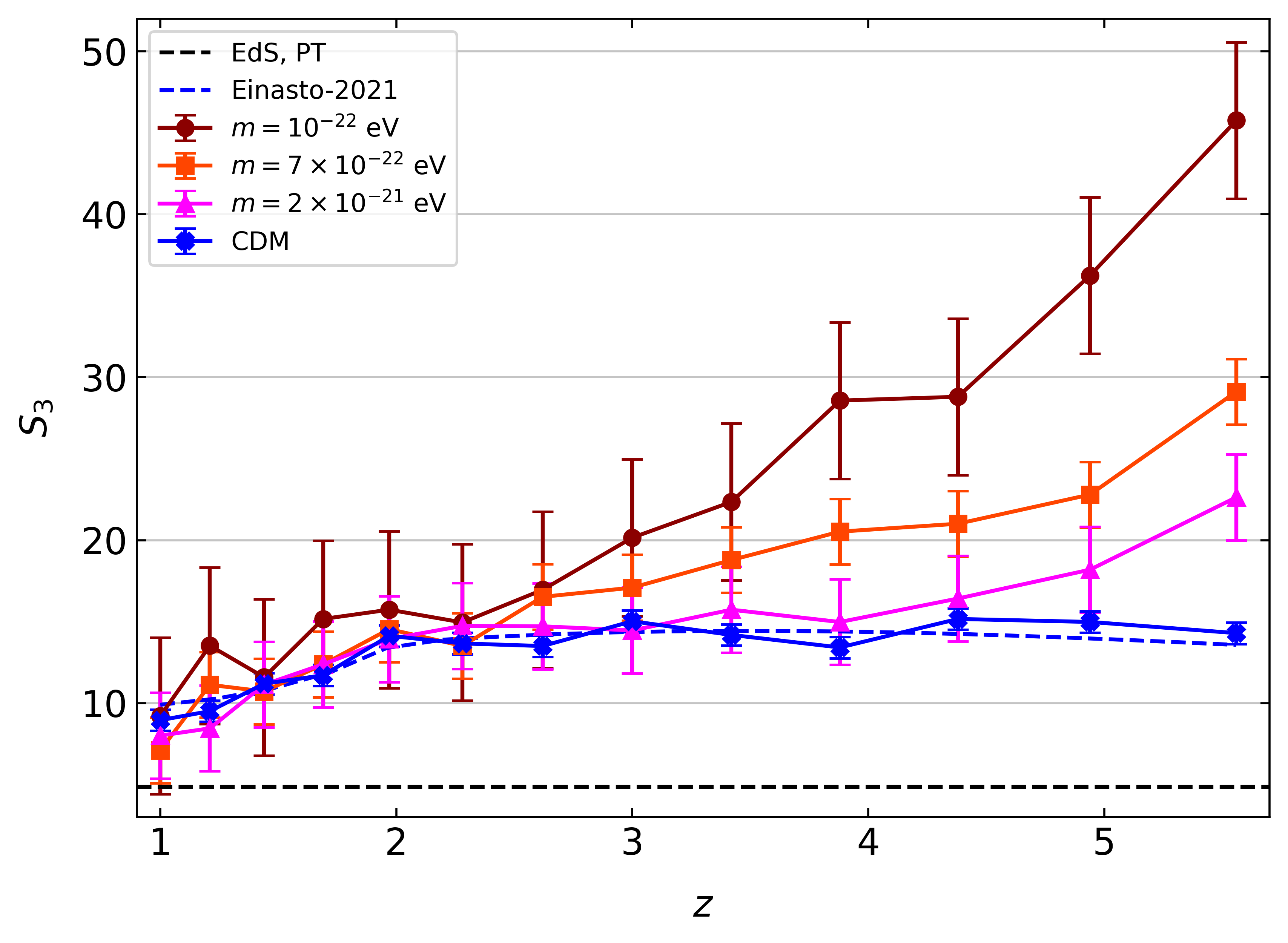
Fig. 5: Skewness \(S_3\) of overdensity PDFs for the \(N\)-body CDM and cFDM runs with \(1024^3\) resolution and \(L_{\text{box}} = 40\ h^{-1}\)Mpc across redshifts \(z\sim 1.0-5.6\). Cosmologies are differentiated by color as shown in the legend. There is no conditioning on cosmic environment. Error estimates from jackknife resampling with \(4^3\) subboxes are marked. The prediction \(S_3 = 34/7\) by Peebles (1980), based on linear PT, for the Einstein-de Sitter (EdS) model (for which \(\Omega_m = 1.0\)) is shown for comparison.

For cFDM, we find that the \(S_3\) estimates are systematically higher than the CDM ones, especially at higher redshift. At \(z=5.6\), the fractional difference in \(S_3\) between \(m=10^{-22}\) eV cFDM and CDM is \((S_3^{10^{-22}\ \mathrm{eV}}-S_3^{\mathrm{CDM}})/S_3^{\mathrm{CDM}} = 2.20 \pm 0.35\), which is different from zero at a level of \(\sim 6 \sigma\).

The fact that \(S_3\) is lower for power spectra with more small-scale fluctuations (CDM) than those with fewer small-scale fluctuations (cFDM) has already been theorised by Bernardeau et al. (2002) using the following argument: Dating back to earlier works such as Bernardeau & Kaufman (1995), it has been noted that the dependence of skewness with the shape of the power spectrum comes from a mapping between Lagrangian space, in which the initial size of the perturbation is determined, and Eulerian space. For a given filtering scale \(R\), overdense regions with \(\delta > 0\) come from the collapse of regions that had initially a larger size while underdense regions with \(\delta < 0\) come from initially smaller regions. In cFDM that has a lack of small coherent regions in the primordial density field, the asymmetry between under- and overdense regions in the evolved density field is greater than in CDM. In Fig. 5, this effect on the skewness \(S_3\) is quantified. In cFDM, non-linear structure formation, e.g. halo mass assembly (Khimey et al. 2021) proceeds faster than in CDM. In the range \(z\sim 2.5-5.0\) where the CDM evolutionary track is around its plateau for the chosen smoothing length \(R\), cFDM is thus already past its plateau and \(S_3\) decreases monotonically with cosmic time before flattening off at \(z\sim 1.0\).

Halo Mass Distributions

According to standard theories of structure formation, DM halos play a crucial role in galaxy formation. However, cosmic environments co-determine the formation of galaxies not least because of large-scale tidal forces. For instance, the enhancement in clustering induced by correlations between halo assembly history and large-scale environment at fixed halo mass is readily observed in cosmological simulations yet difficult to detect in observations, called halo & galaxy assembly bias (Sunayama et al. 2022. Here, we investigate the differences in the halo population across the cosmic web components which in turn are suggestive of variations with large-scale environment in the population of galaxies and their properties.

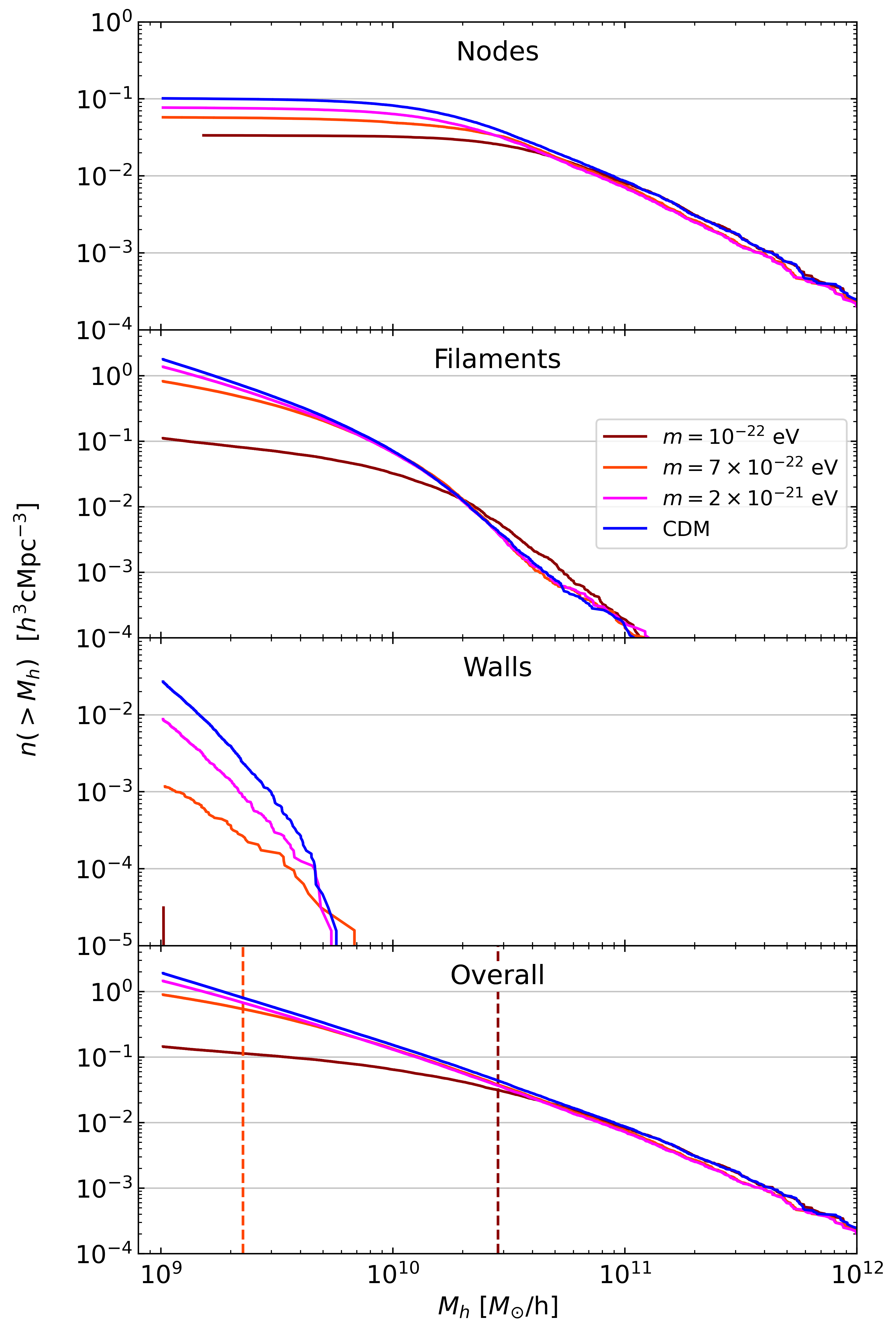
Fig. 6: Cumulative halo mass functions (cHMFs) for the \(N\)-body CDM and cFDM runs with \(1024^3\) resolution and \(L_{\text{box}} = 40\ h^{-1}\)Mpc at redshift \(z=3.9\), split according to the NEXUS+ environment in which the halo resides, indicated for each panel. The last row shows the overall cHMFs; vertical dashed lines denote the half-mode mass \(M_{1/2}\) (Marsh 2016) of the \(m=10^{-22}\) eV and the \(m=7\times 10^{-22}\) eV models (for \(m=2\times 10^{-21}\) eV cFDM, \(M_{1/2} = 5.77 \times 10^8 \ h^{-1} M_{\odot}\) is off-scale).

Fig. 6 shows the cumulative halo mass function (cHMF) segmented into cosmic web environments, at \(z=3.9\). We find that the most massive halos across all cosmologies are exclusively found in node regions, especially beyond \(M_h \sim 10^{11} \ h^{-1} M_{\odot}\). The vast majority of halos that are not located in nodes are filament halos, which start to dominate the cHMF below about \(M_h\sim 2\times 10^{10}\ h^{-1} M_{\odot}\). Halos in walls and voids (not shown) represent a substantial share of the halo population only at the lowest resolved masses below \(M_h \sim 2\times 10^{9} \ h^{-1} M_{\odot}\). In particular, since this behavior is exhibited regardless of cosmology it implies that very few luminous galaxies and quasars are and will be observed in cosmic sheets with current and upcoming galaxy/QSO redshift surveys such as SDSS SEQUELS (Myers et al. 2015), the DESI Bright Galaxy Survey (BGS) and JWST Advanced Deep Extragalactic Survey (JADES).

In analogy to WDM (Schneider et al. 2012) and bona-fide FDM HMF analyses (May & Springel 2022), we confirm that cFDM cosmologies have fewer small-mass halos compared to CDM but here we quantify the environment-conditioned cHMFs. All node-, filament- and wall-conditioned cHMFs exhibit a strong suppression in cFDM cosmologies, but for some environments this occurs well above the half-mode mass \(M_{1/2}\) (Marsh 2016). As seen in Fig. 6 at \(z=3.9\), the node-conditioned cHMF of the \(m=7\times 10^{-22}\) eV model exhibits a \(50\)% reduction below a mass of \(M_h \sim 10^{10} \ h^{-1} M_{\odot}\) while the half-mode mass is \(M_{1/2} = 2.3\times 10^{9} \ h^{-1} M_{\odot}\). For wall halos in \(m=7\times 10^{-22}\) eV cFDM, we observe a \(>50\)% reduction below a mass of \(M_h \sim 4 \times 10^{9} \ h^{-1} M_{\odot}\). Thus, if the given environment is not dominant on the mass scale considered, the cFDM suppression can turn out stronger than naively expected from \(M_{1/2}\).

We also observe that for walls (subdominant environment), the cFDM suppression of the conditioned cHMFs is stronger than for nodes and filaments. At the smallest resolved halo mass of \(M_{\text{min}} \sim 10^{9} \ h^{-1} M_{\odot}\), compared to CDM the \(m=7\times 10^{-22}\) eV cFDM model exhibits a \(\sim 1.1\) dex suppression in the wall-conditioned cHMF. For both the node-conditioned and filament-conditioned HMF, however, the corresponding suppression is less than \(\sim 0.5\) dex. In simple terms, walls and voids (not shown) are disproportionately more devoid of halos in cFDM cosmologies than in CDM. In addition, the filament-conditioned cHMF of the rather extreme \(m=10^{-22}\) eV model features a slight enhancement above \(M_h \sim 2 \times 10^{10} \ h^{-1} M_{\odot}\), though due to the smallness of this effect we refrain from attributing physical significance to it.